
library(arrow)
library(dplyr)
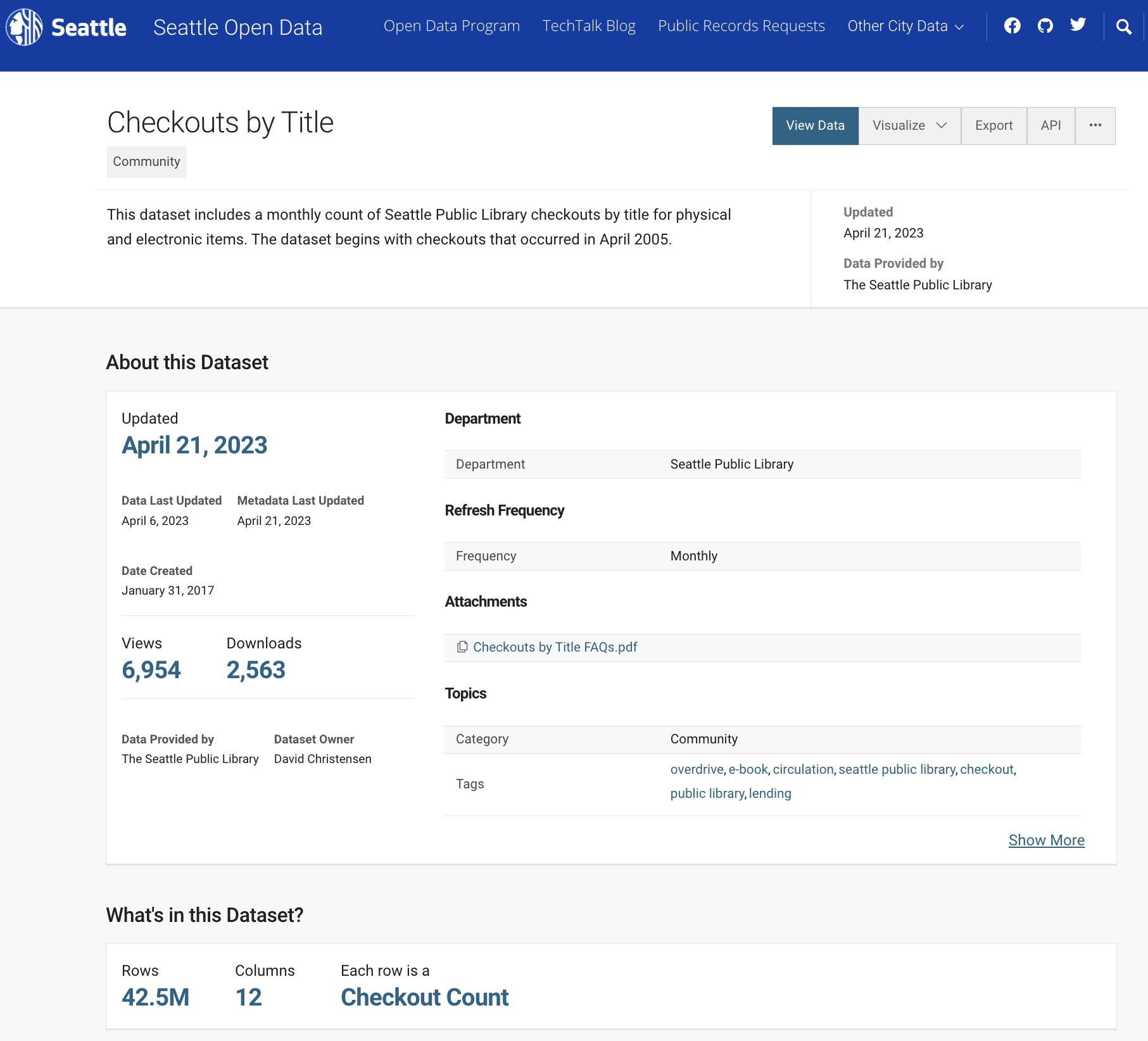
seattle_csv <- open_dataset(here::here("data/seattle-library-checkouts.csv"),
format = "csv")
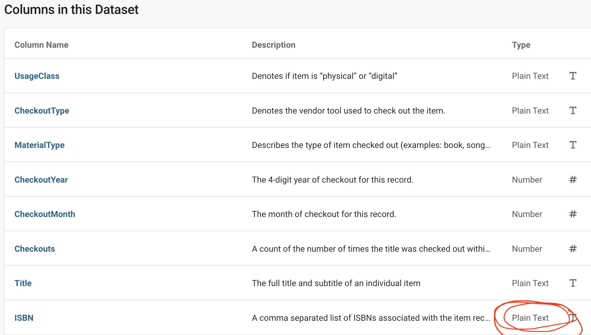
seattle_csvFileSystemDataset with 1 csv file
UsageClass: string
CheckoutType: string
MaterialType: string
CheckoutYear: int64
CheckoutMonth: int64
Checkouts: int64
Title: string
ISBN: null
Creator: string
Subjects: string
Publisher: string
PublicationYear: string