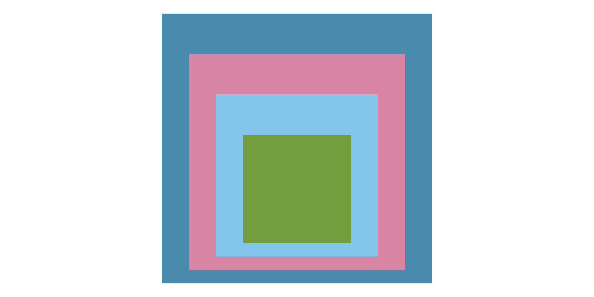
Steal like an Rtist: Creative Coding in R

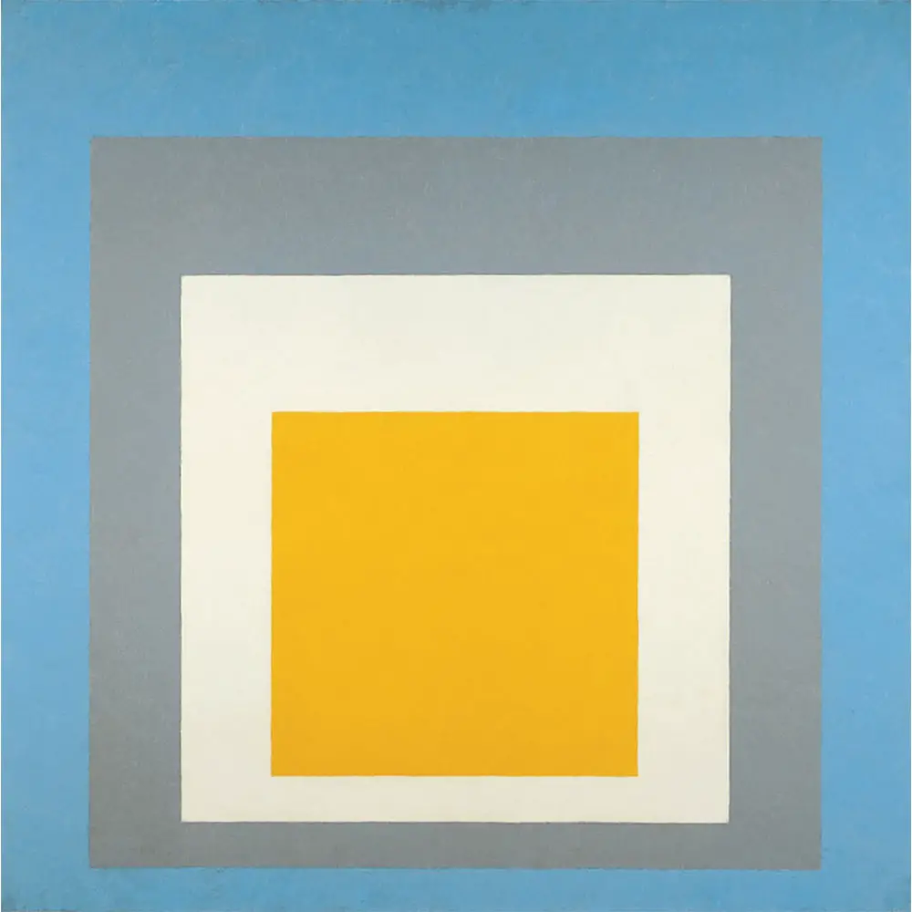
Homage to the Square
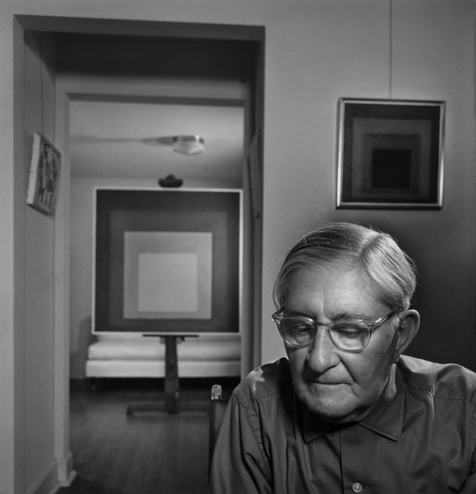
Josef Albers

Ijeamaka Anyene Fumagalli and Sharla Gelfand

posit::conf(2023)

Homage to the Square – Ascending, 1953

Josef Albers, 1966, by Yousuf Karsh

Josef Albers was a prominent German artist in the 20th century

Educator at Bauhaus, Black Mountain College in North Carolina, and Yale

Expert at studying and teaching color

Series of paintings from 1950 to 1976 focused on color

Recreating the one pictured here

 

Thousands of paintings

Applied color directly from the tube with a palette knife, not traditionally “painted”

All of the colors, etc, codified on the backs of the paintings

Exploring color and relationships, subjectivity

Homage to the Square – Ascending, 1953

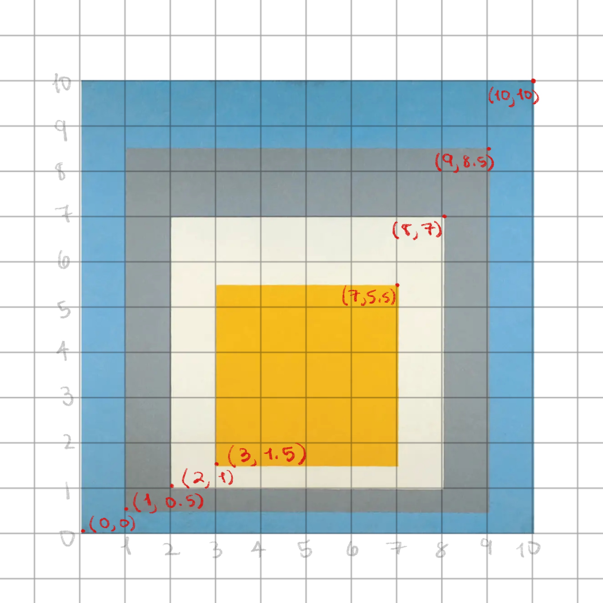
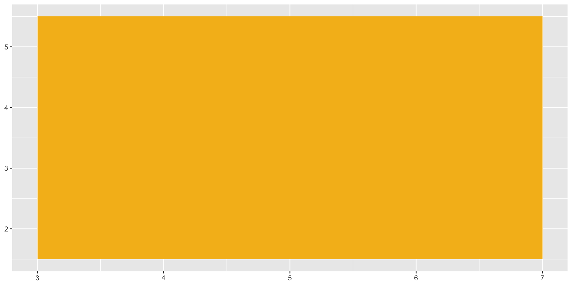
Creating a rectangle in {ggplot2}

geom_rect()

Use arguments to map data to visual properties

• xmin, xmax: minimum and maximum x values
• ymin, ymax: minimum and maximum y values
• fill: color

Creating a rectangle in {ggplot2}

geom_rect()

library(ggplot2)

ggplot() +
  geom_rect(
    aes(
      xmin = 3, xmax = 7,
      ymin = 1.5, ymax = 5.5
    ),
    fill = "#F5BB1D"
  )

Recreate

library(dplyr)

homage <- tribble(
  ~x0, ~y0, ~size,    ~color,
    0,   0,    10, "#5A9CBA",
    1, 0.5,     8, "#919EA3",
    2,   1,     6, "#F1EFDF",
    3, 1.5,     4, "#F5BB1D"
  ) %>%
  mutate(
    x1 = x0 + size,
    y1 = y0 + size
  )

homage

Recreate

library(dplyr)

homage <- tribble(
  ~x0, ~y0, ~size,    ~color,
    0,   0,    10, "#5A9CBA",
    1, 0.5,     8, "#919EA3",
    2,   1,     6, "#F1EFDF",
    3, 1.5,     4, "#F5BB1D"
  ) %>%
  mutate(
    x1 = x0 + size,
    y1 = y0 + size
  )

homage

Recreate

library(dplyr)

homage <- tribble(
  ~x0, ~y0, ~size,    ~color,
    0,   0,    10, "#5A9CBA",
    1, 0.5,     8, "#919EA3",
    2,   1,     6, "#F1EFDF",
    3, 1.5,     4, "#F5BB1D"
  ) %>%
  mutate(
    x1 = x0 + size,
    y1 = y0 + size
  )

homage

Recreate

library(dplyr)

homage <- tribble(
  ~x0, ~y0, ~size,    ~color,
    0,   0,    10, "#5A9CBA",
    1, 0.5,     8, "#919EA3",
    2,   1,     6, "#F1EFDF",
    3, 1.5,     4, "#F5BB1D"
  ) %>%
  mutate(
    x1 = x0 + size,
    y1 = y0 + size
  )

homage

Recreate

library(dplyr)

homage <- tribble(
  ~x0, ~y0, ~size,    ~color,
    0,   0,    10, "#5A9CBA",
    1, 0.5,     8, "#919EA3",
    2,   1,     6, "#F1EFDF",
    3, 1.5,     4, "#F5BB1D"
  ) %>%
  mutate(
    x1 = x0 + size,
    y1 = y0 + size
  )

homage

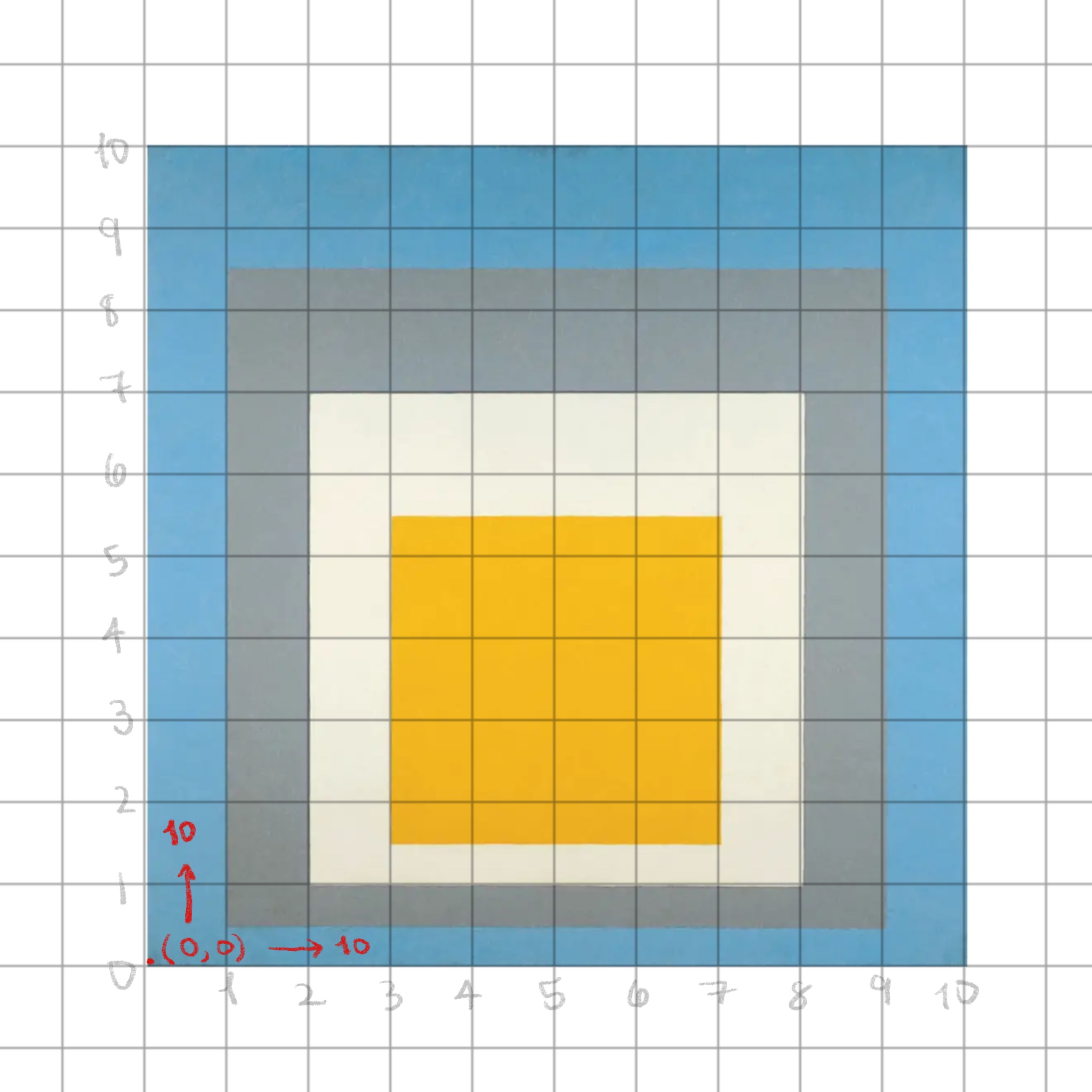
Recreate

library(dplyr)

homage <- tribble(
  ~x0, ~y0, ~size,    ~color,
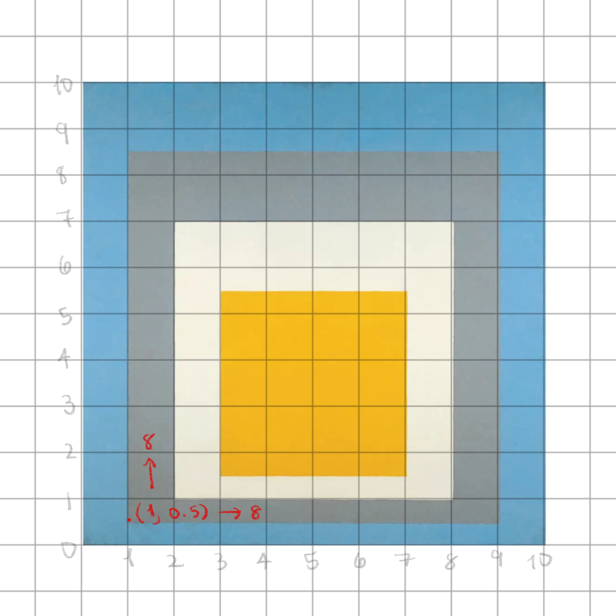
    0,   0,    10, "#5A9CBA",
    1, 0.5,     8, "#919EA3",
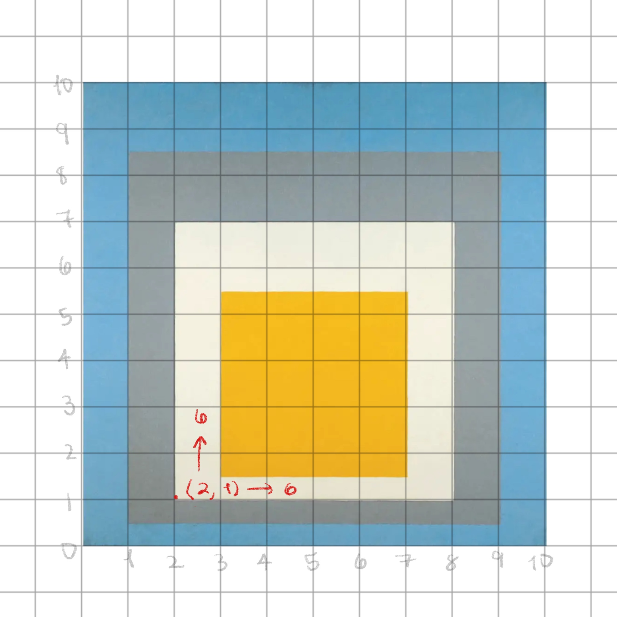
    2,   1,     6, "#F1EFDF",
    3, 1.5,     4, "#F5BB1D"
  ) %>%
  mutate(
    x1 = x0 + size,
    y1 = y0 + size
  )

homage

# A tibble: 4 × 6
     x0    y0  size color      x1    y1
  <dbl> <dbl> <dbl> <chr>   <dbl> <dbl>
1     0   0      10 #5A9CBA    10  10  
2     1   0.5     8 #919EA3     9   8.5
3     2   1       6 #F1EFDF     8   7  
4     3   1.5     4 #F5BB1D     7   5.5

Recreate

homage_p <- ggplot(homage) +
  geom_rect(aes(
    xmin = x0,
    xmax = x1,
    ymin = y0,
    ymax = y1,
    fill = color
  ))

homage_p

Recreate

homage_p <- ggplot(homage) +
  geom_rect(aes(
    xmin = x0,
    xmax = x1,
    ymin = y0,
    ymax = y1,
    fill = color
  ))

homage_p

ggplot2 thinks color is a categorical variable that needs to be represented by a fill color

Recreate

homage_p <- ggplot(homage) +
  geom_rect(aes(
    xmin = x0,
    xmax = x1,
    ymin = y0,
    ymax = y1,
    fill = color
  )) +
  scale_fill_identity()

homage_p

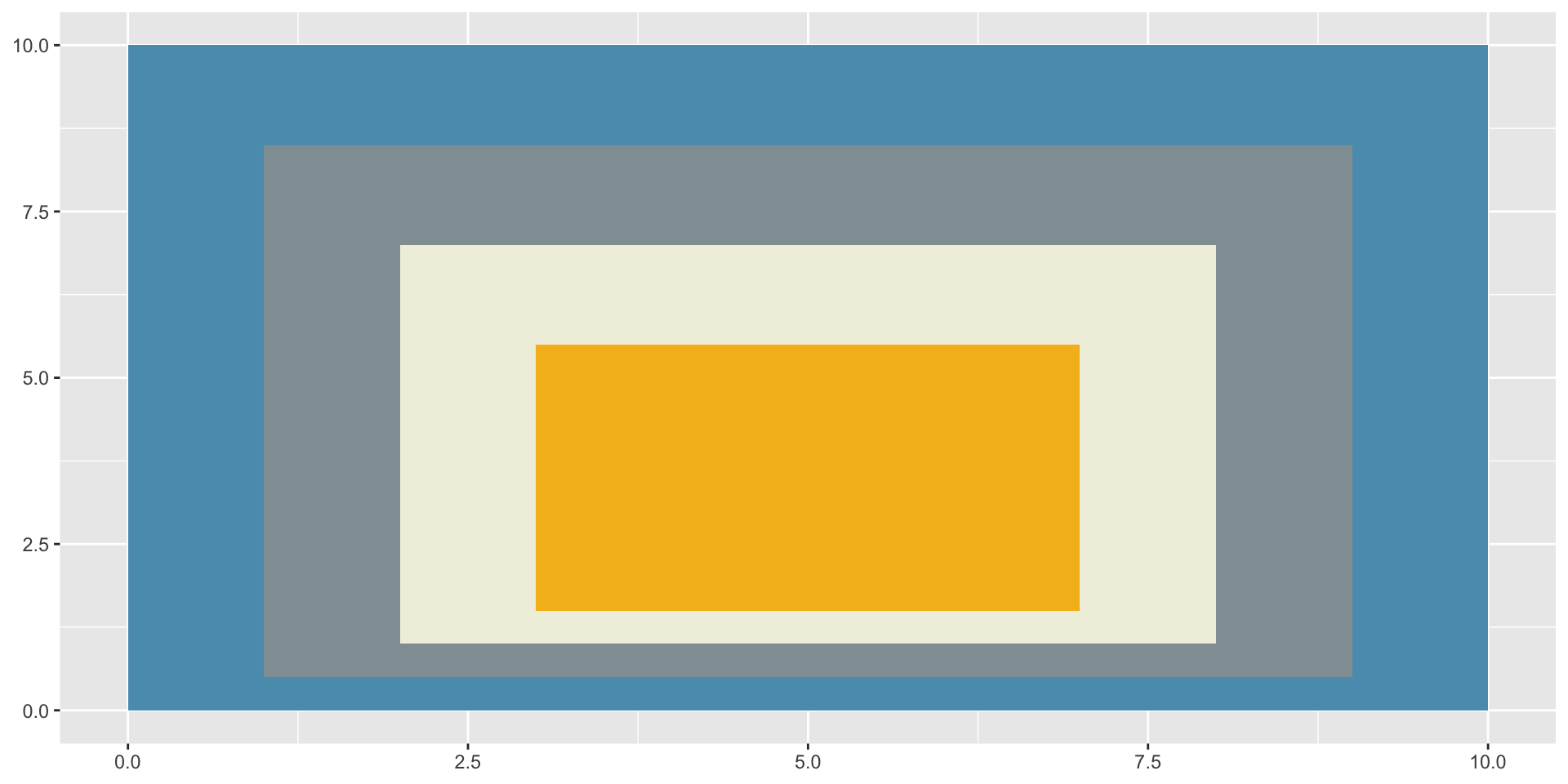
scale_fill_identity() tells ggplot2 the variable in color is a color value it can use directly, not a categorical variable that needs to be represented by a fill color

Recreate

homage_p <- ggplot(homage) +
  geom_rect(aes(
    xmin = x0,
    xmax = x1,
    ymin = y0,
    ymax = y1,
    fill = color
  )) +
  scale_fill_identity() +
  coord_fixed()

homage_p

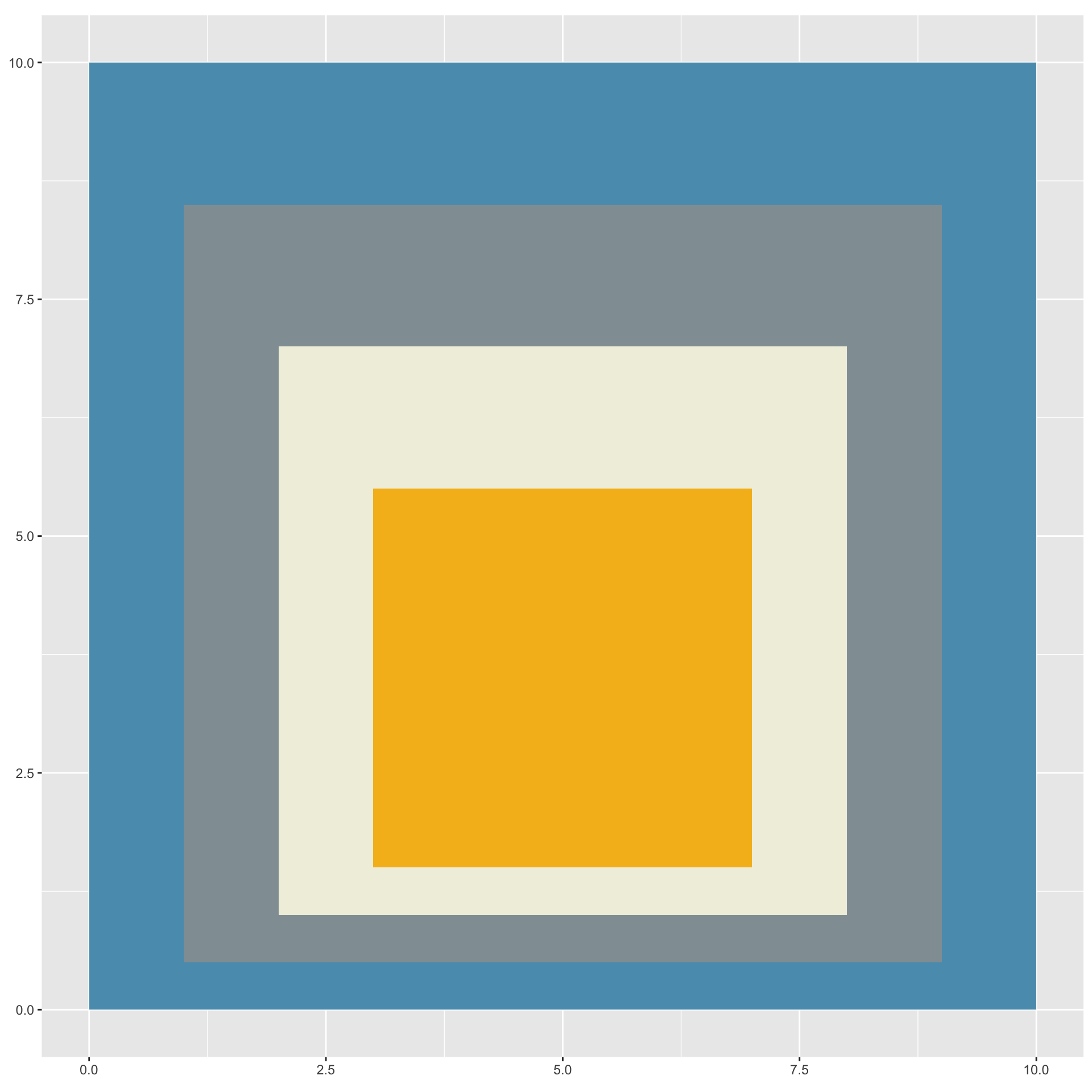
coord_fixed() sets a fixed coordinate system, with an aspect ratio of 1, to ensure one unit on the x-axis is the same as one unit on the y-axis (aka: a square is a square)

Recreate

homage_p <- ggplot(homage) +
  geom_rect(aes(
    xmin = x0,
    xmax = x1,
    ymin = y0,
    ymax = y1,
    fill = color
  )) +
  scale_fill_identity() +
  coord_fixed() +
  theme_void()

homage_p

theme_void() is a completely empty theme, creating a blank canvas for us to work on

Recreate

homage_p <- ggplot(homage) +
  geom_rect(aes(
    xmin = x0,
    xmax = x1,
    ymin = y0,
    ymax = y1,
    fill = color
  )) +
  scale_fill_identity() +
  coord_fixed(expand = FALSE) +
  theme_void()

homage_p

coord_fixed() with expand = FALSE removes any margin

Save your work

go to Rstudio

ggsave("homage.png",
  homage_p,
  bg = "black"
)

vs according to the actual dimensions of the work

ggsave("homage_square.png",
  homage_p,
  width = 5,
  height = 5,
  bg = "black"
)

Recreation done!

Homage to the Square – Ascending, 1953

Homage to the Square – Ascending, recreation, 2023

What is generative art?

“Generative art operates within a rule structure but has an element of chance that is crucial to what many artists enjoy about it. The final work is partly produced by an autonomous system, which may be strictly regulated by the rules or operate within parameters.”

— Charlotte Kent, Beyond the Janus-Faced Typologies of Art and Technology

Done with recreation, how do we move on to remix it? Create a generative art system

What is generative art?

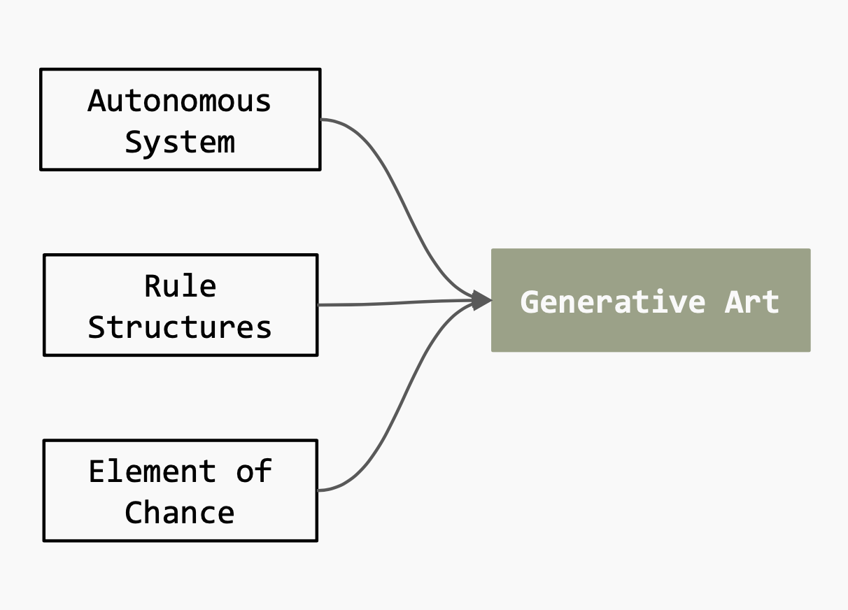
Remix time! Creating a small system

make_homage <- function(colors = c("#5A9CBA", "#919EA3", "#F1EFDF", "#F5BB1D")) {
  tribble(
   ~x0, ~y0, ~size,
     0,   0,    10,
     1, 0.5,     8,
     2,   1,     6,
     3, 1.5,     4
   ) %>%
    mutate(
      x1 = x0 + size,
      y1 = y0 + size,
      color = sample(colors, size = 4)
    ) %>%
    ggplot() +
    geom_rect(aes(
      xmin = x0, xmax = x1,
      ymin = y0, ymax = y1,
      fill = color
    )) +
    scale_fill_identity() +
    coord_fixed() +
    theme_void()
}

Remix time! Creating a small system

make_homage()

make_homage()

Each call of the function creates a different output, since the order of the colors is sampled

set.seed()

What if you like an output?

Setting a seed controls the state of the random number generator in R

set.seed(1234)

make_homage()

set.seed(1234)

make_homage()

Setting the same seed creates the same output, since the random number generator is at the same “state” each time the sample is taken

Your turn!

1. Open the file exercises/02-homage-to-the-square/exercise-1.Rmd
2. Update the function make_my_homage() to take a seed argument, and set the seed in the body of the function
3. Verify that running make_my_homage() with the same seed creates the same output, and that with a different seeds creates different outputs
4. Share an output and the seed that created it in the GitHub discussion for this exercise

05:00

Composition

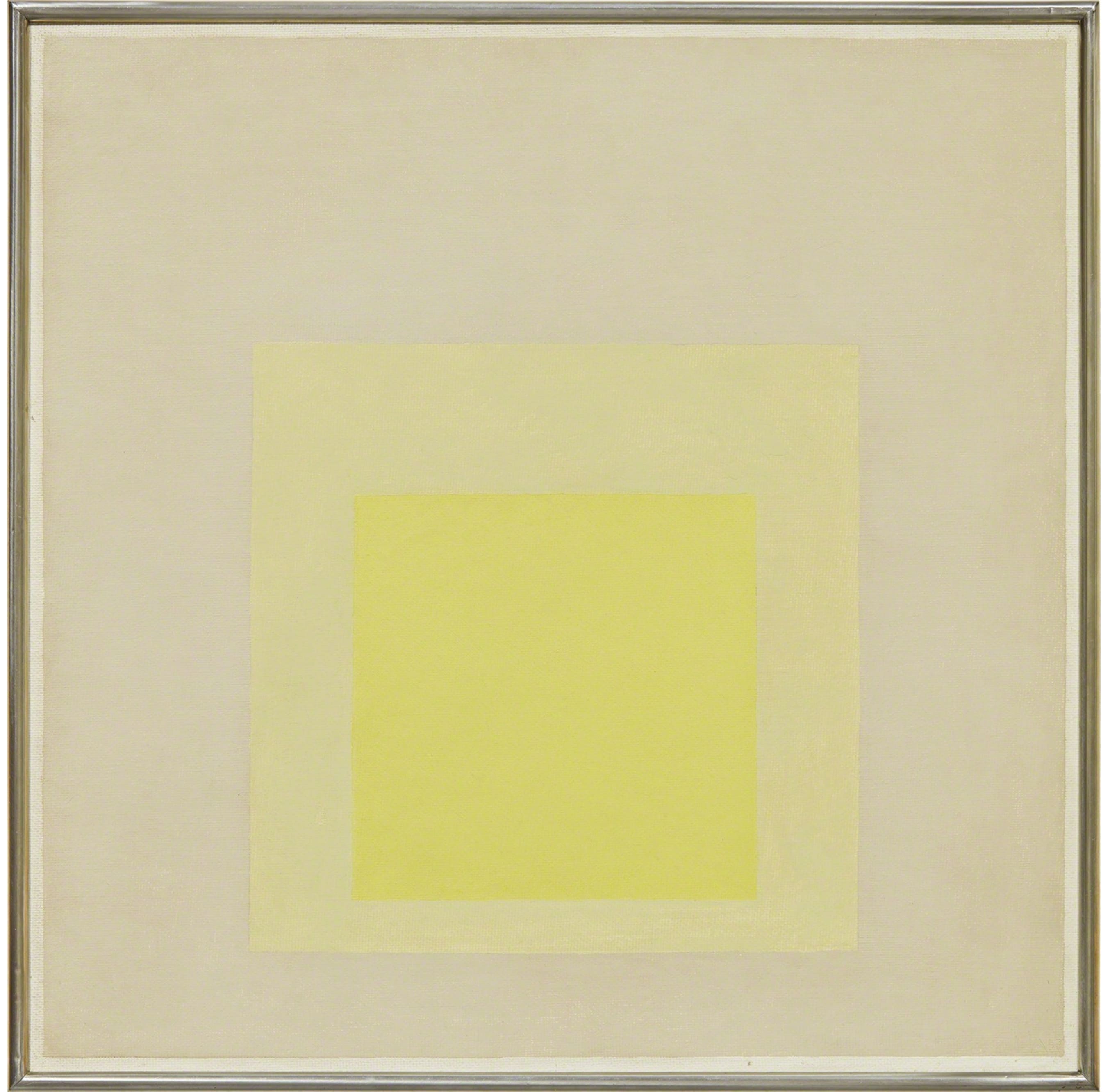
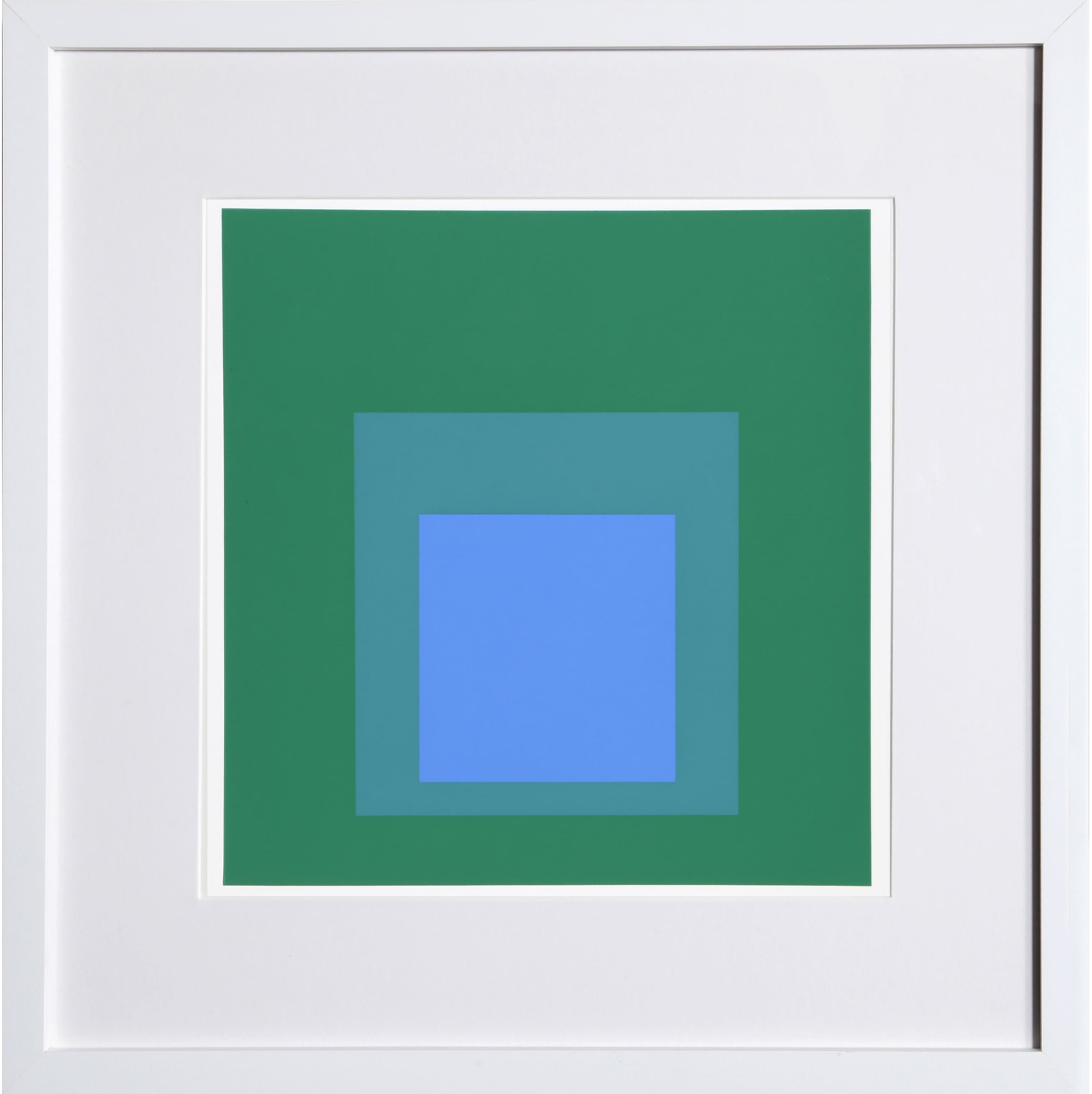
Deliberately simple and consistent in structure, the nested squares were a platform for exploring color.

Homages are all about mutability of color relationships and the malleability of subjective perceptions of colors.

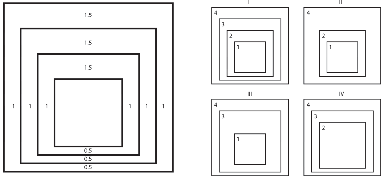
Planes and Frames: Spatial Layering in Josef Albers’ Homage to the Square Paintings, J. Mai, 2016

Series was based on mathematically determined format - we can appreciate this!

Original is top middle - how do different ones affect how we see the piece, how the colors interact? Visual effect

Color

Albers started with neutrals, exploring the relative lightness and darkness of colors

He sought the yellow tint in white, the blue and brown in black -> impurities of white and black on screen vs life

He explored how grey can be violet, how opposite colors accentuate each other, how some colors seem brighter than others

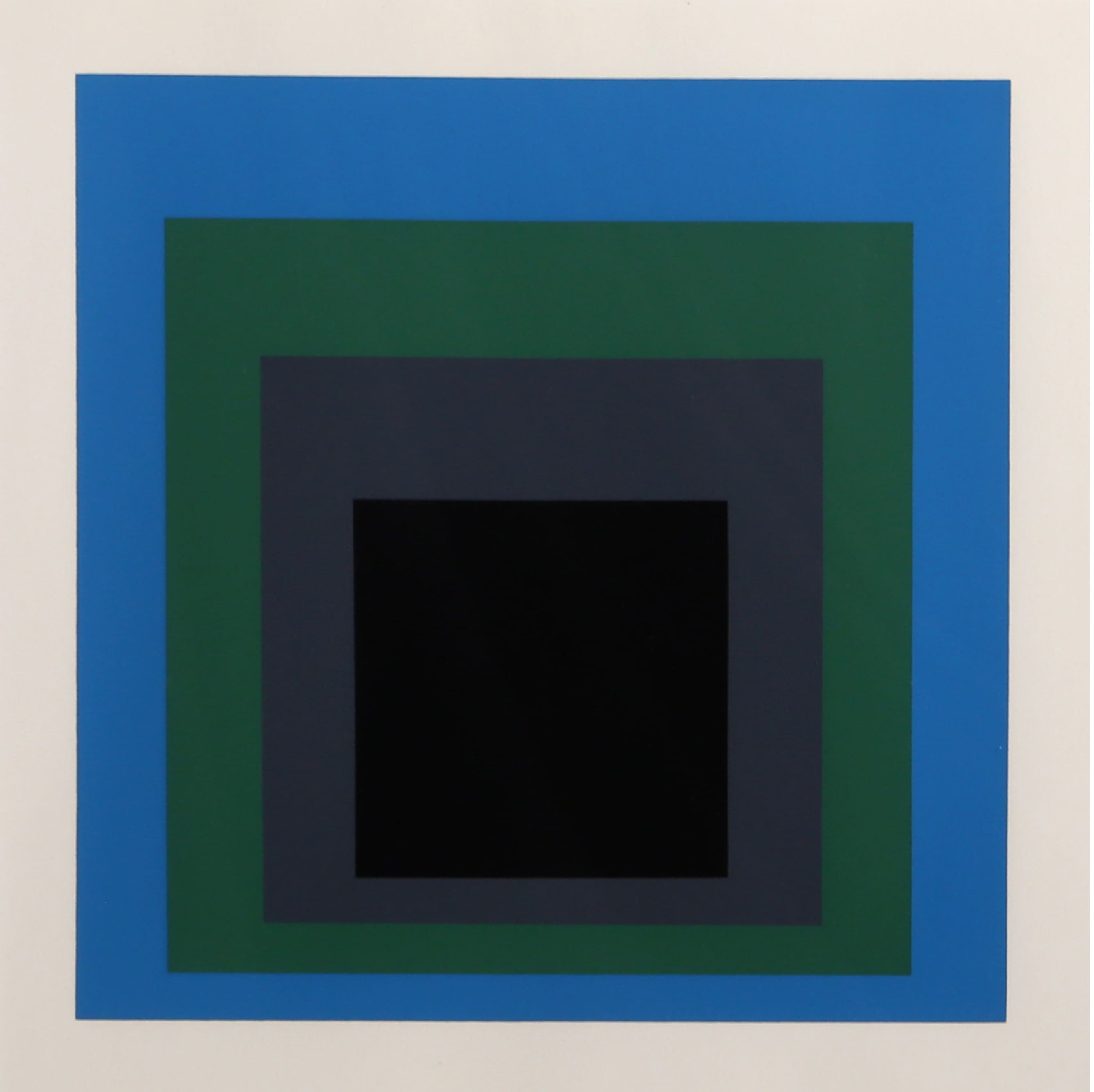
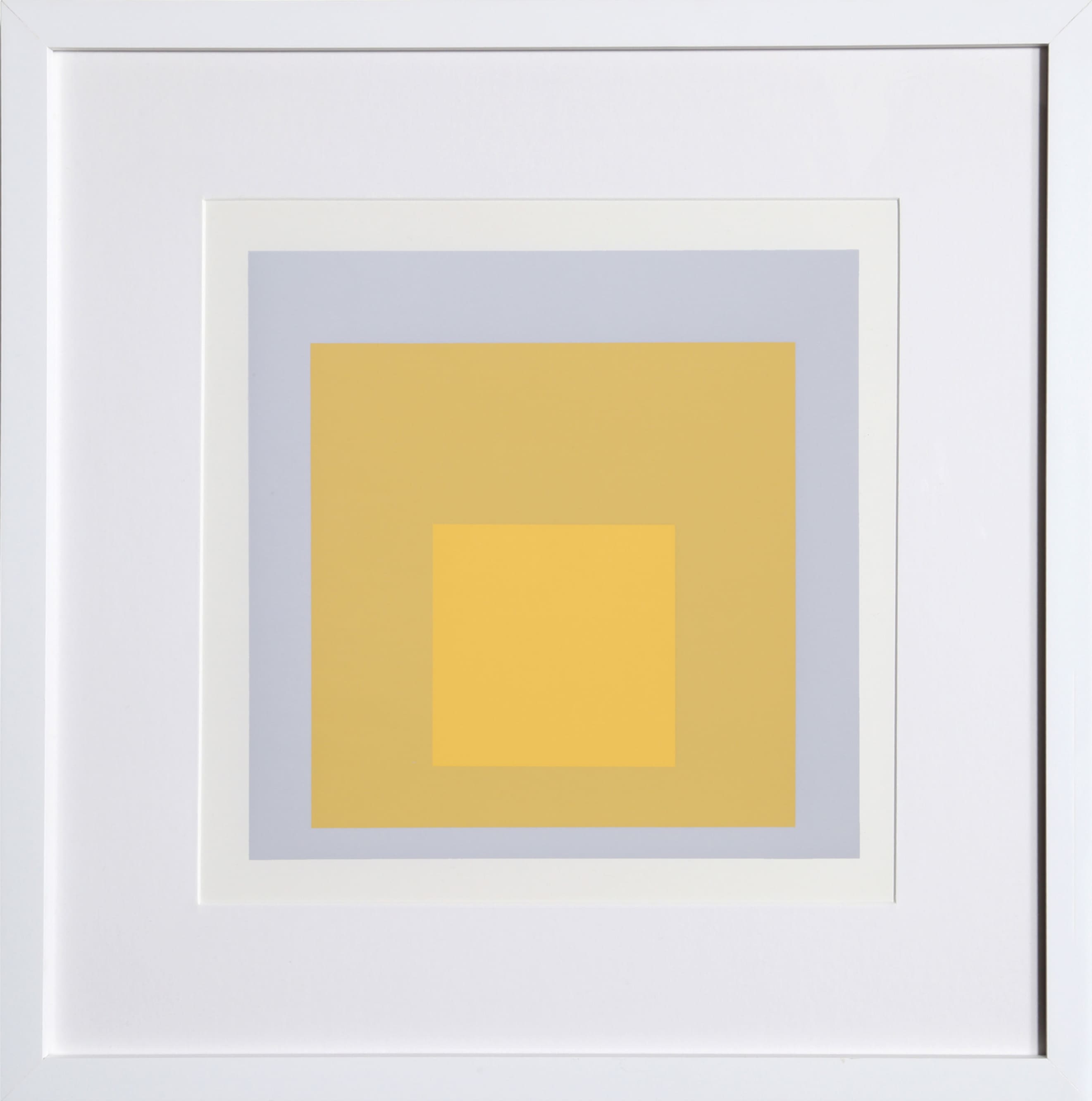
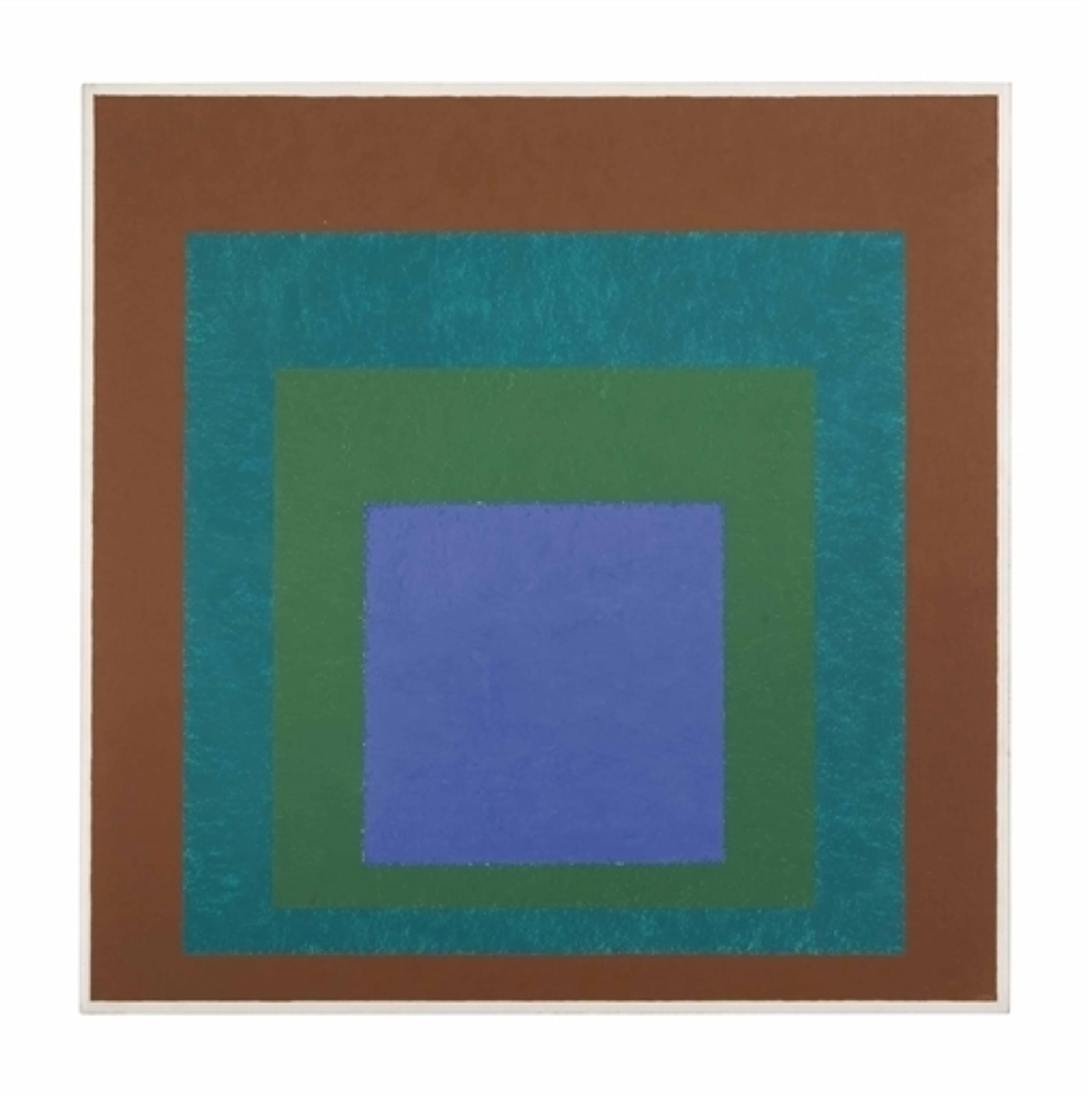
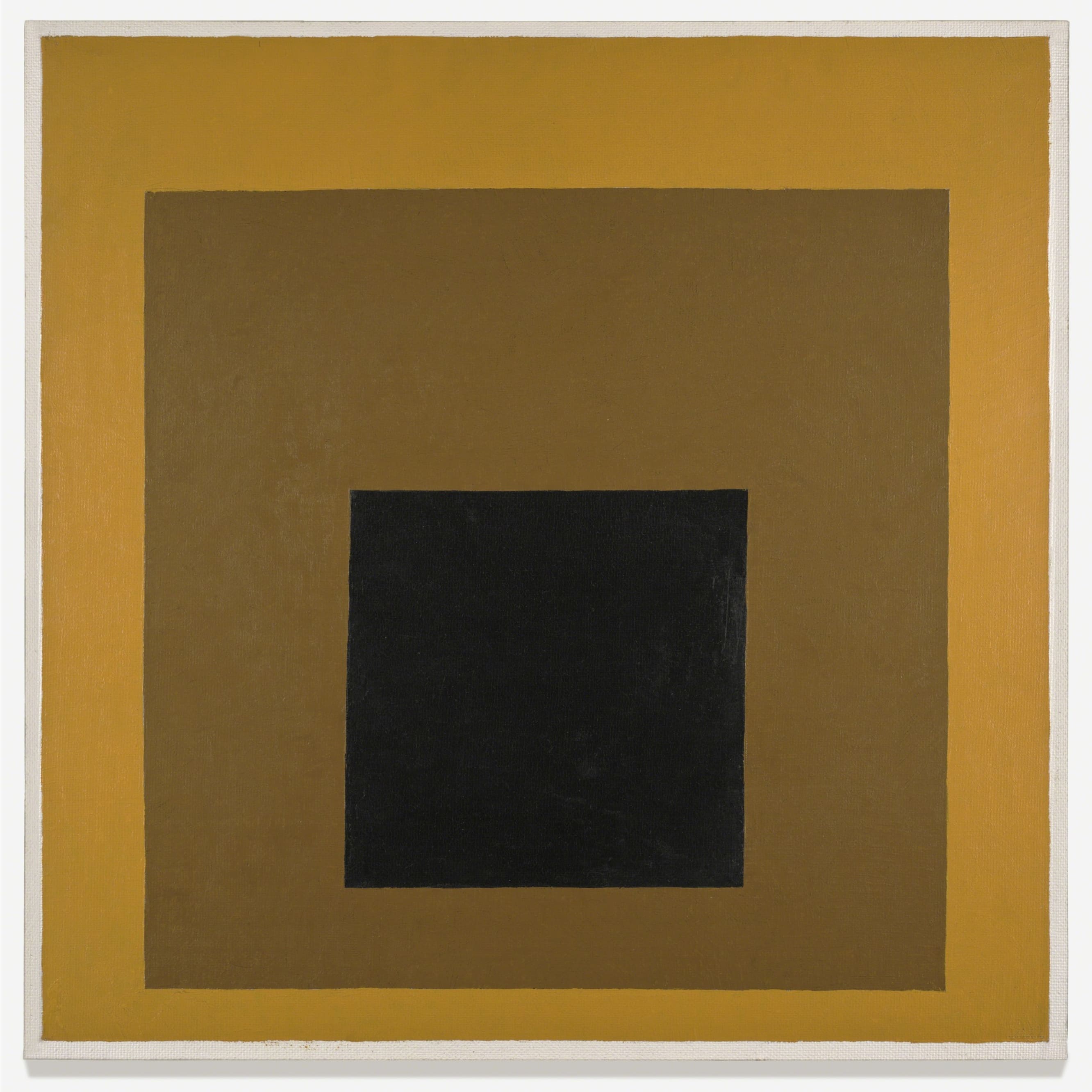
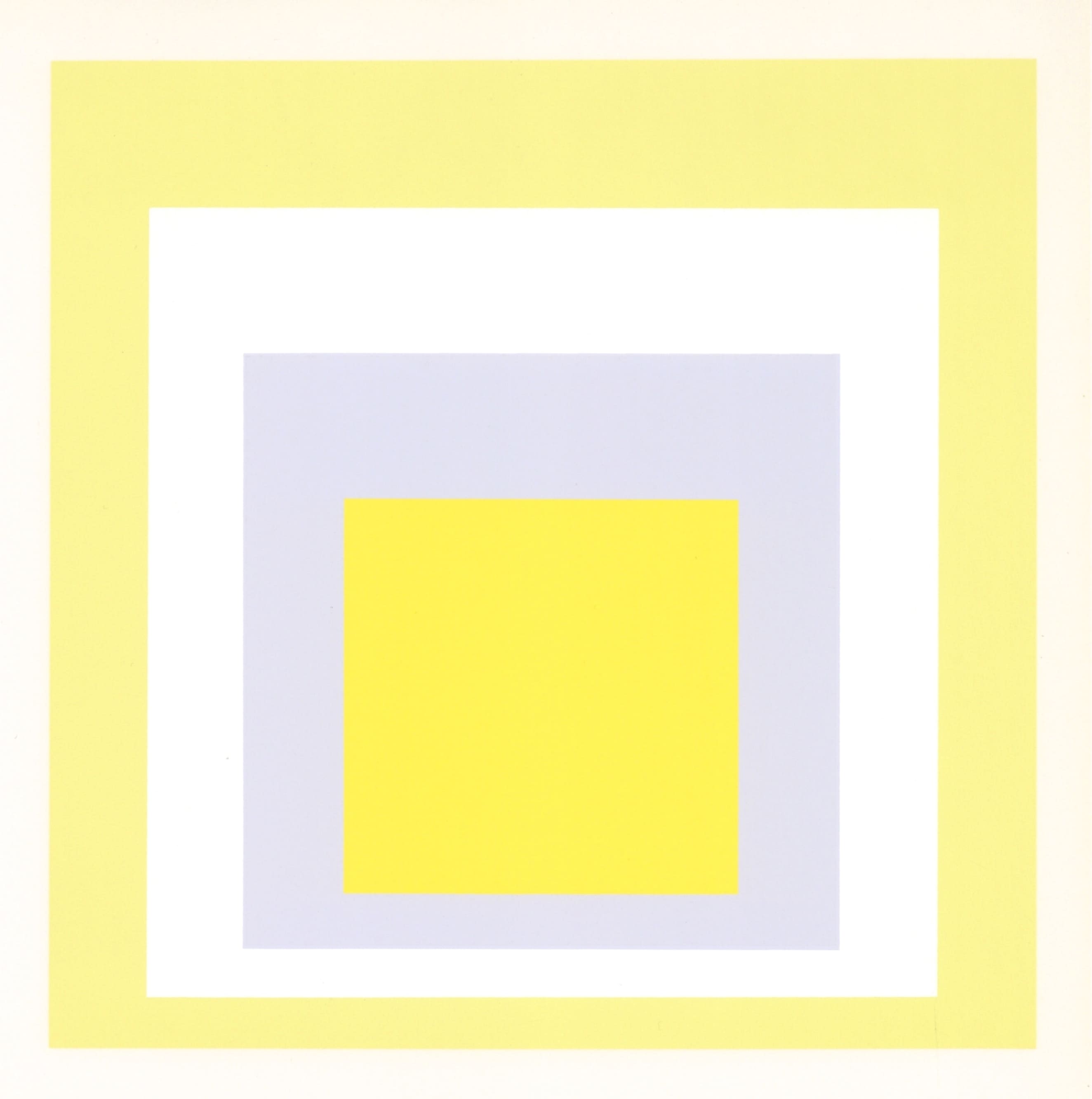
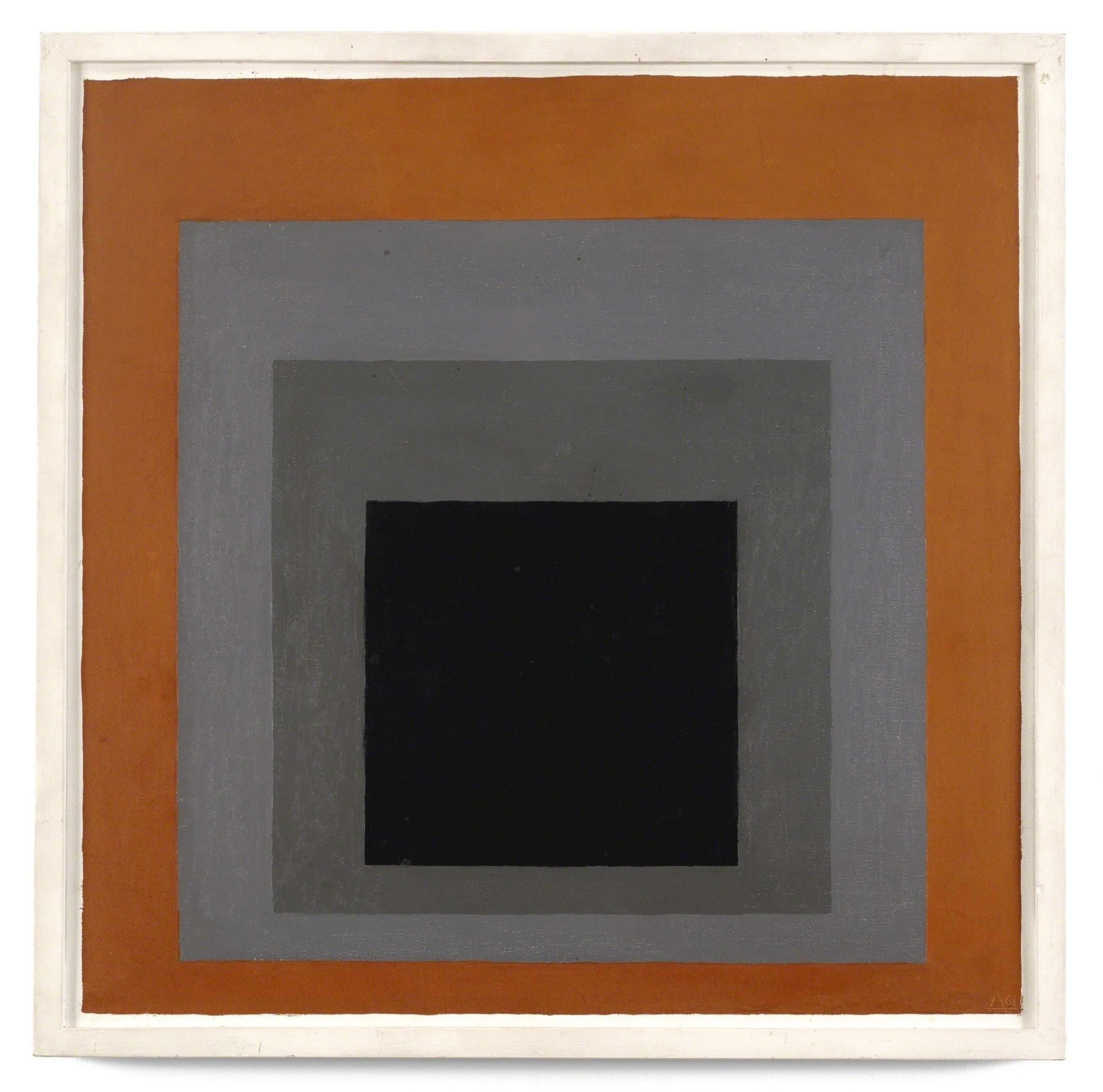
Hex

An opaque but common format of representing color

library(scales)

palette <- c("#4d5a0b", "#f37f92", "#f49346", "#ffcd84")

show_col(palette)

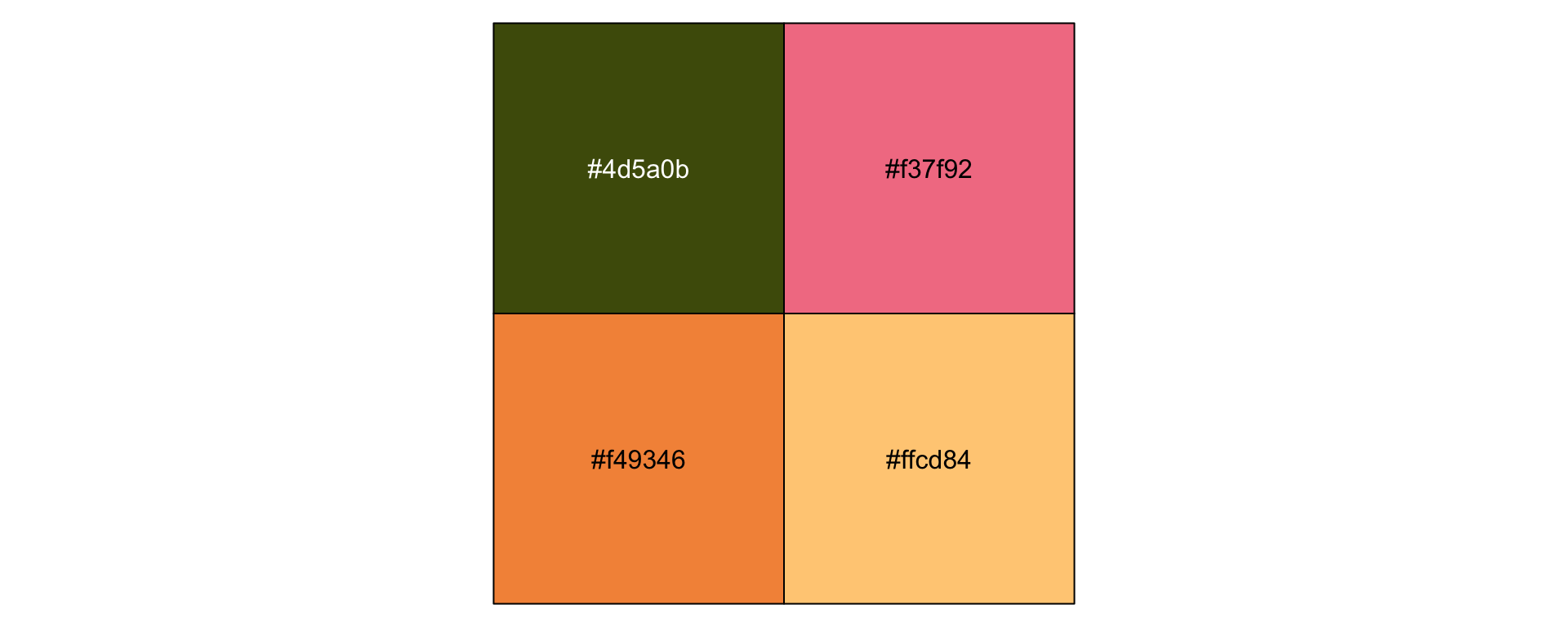
“#5A9CBA” is one of the colors we used before - what is it?

RGB

How much red, green, and blue make up a color (0 to 255)

mystery_color <- "#5A9CBA"

col2rgb(mystery_color)

      [,1]
red     90
green  156
blue   186

What does this actually tell you? It’s not so red, it’s kinda green, and more blue?

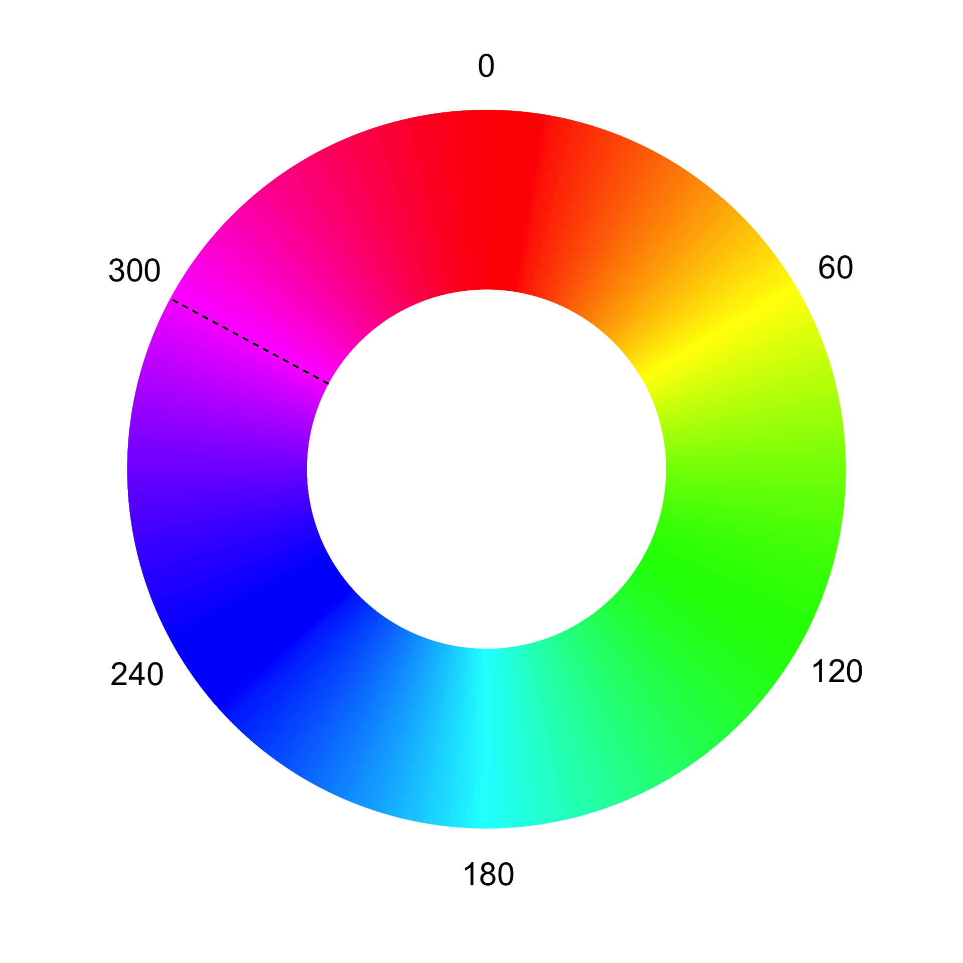
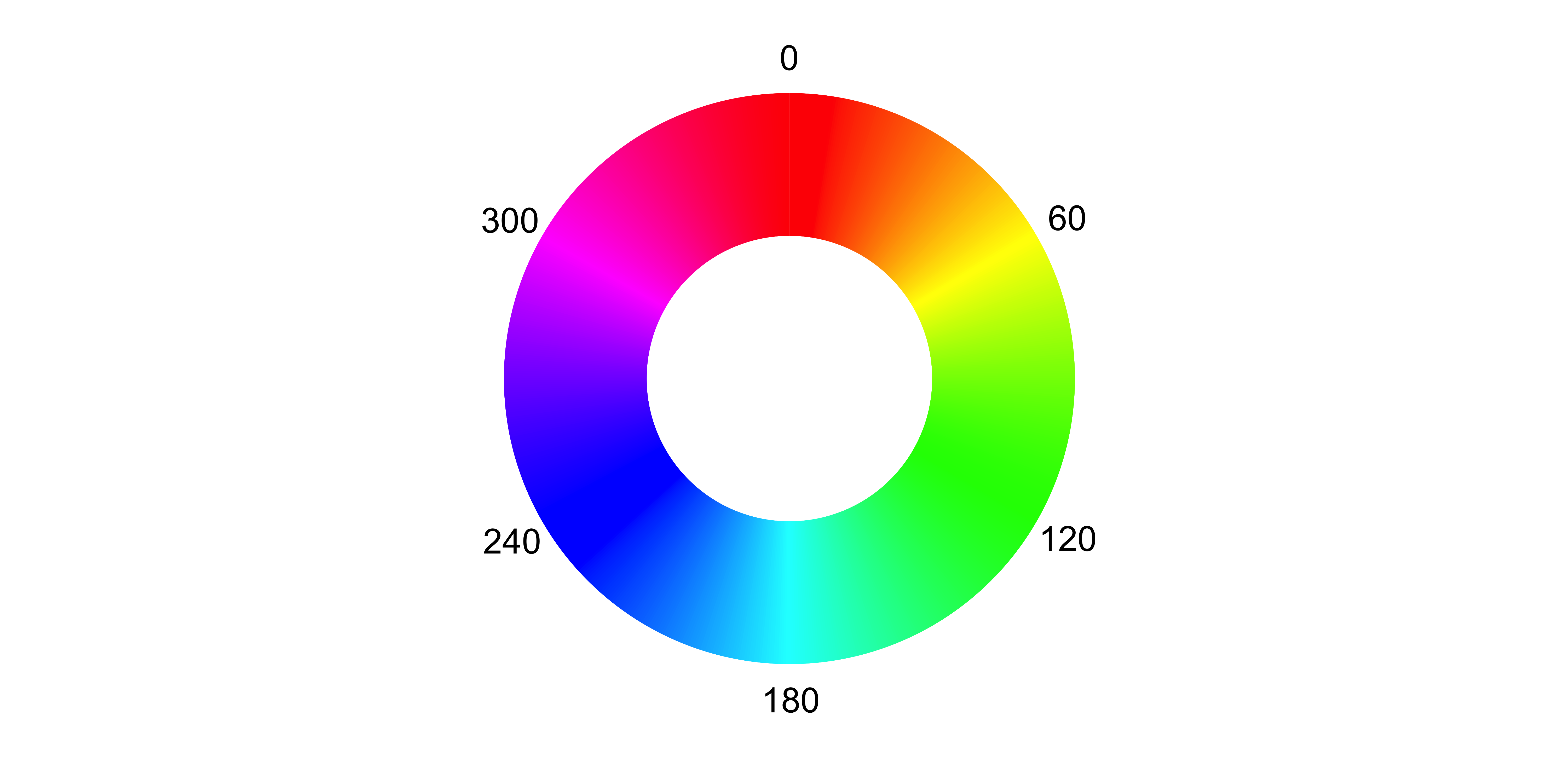
HSL

HSL is a clearer color system that is easier for a human to understand

Also easier to alter colors

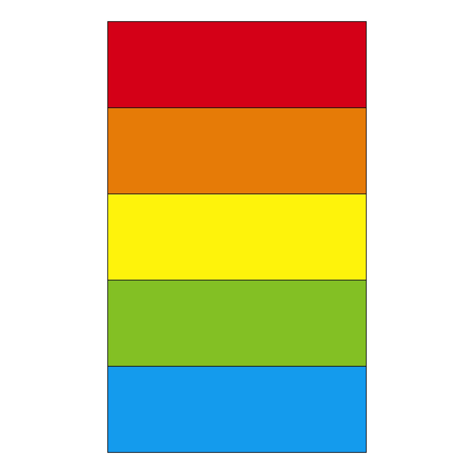
Hue

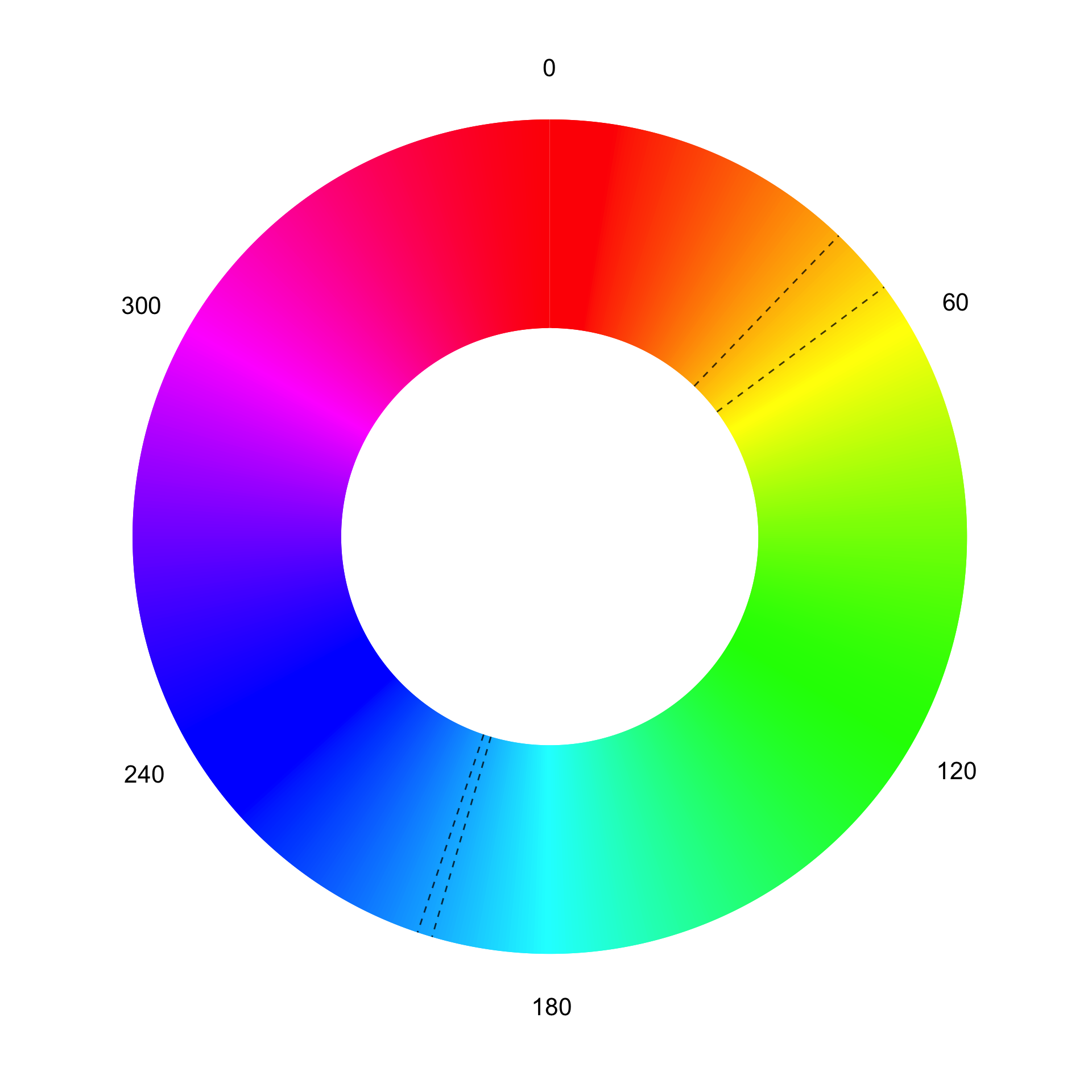
Color on the color wheel

(0 to 360)

Saturation

Vividness, how much of the color is actually present

From grey to full saturation of the color (0% to 100%)

Lightness

How light/bright the color is

From black to white (0% to 100%)

Hue

Hue

library(prismatic)

mystery_color <- color(mystery_color)

color(mystery_color) %>%
  clr_extract_hue()

[1] 198.75

Hue

mystery_color %>%
  clr_rotate(degrees = 100)

<colors>
#C17FAAFF 

Saturation

Same hue and lightness (50%), saturation from 0% to 100%

mystery_color %>%
  clr_extract_saturation()

[1] 41.02564

saturated_color <- mystery_color %>%
  clr_saturate(shift = 0.5)

desaturated_color <- mystery_color %>%
  clr_desaturate(shift = 0.5)

c(saturated_color, mystery_color, desaturated_color) %>%
  color() %>%
  plot()

Saturation

Desaturation generally makes things more interesting… compare to our palette in full saturation

homage[["color"]] %>%
  color() %>%
  clr_saturate(shift = 1) %>%
  plot()

Lightness

Same hue and saturation (50%), lightness from 0% to 100%

mystery_color %>%
  clr_extract_lightness()

[1] 54.11765

lighter_color <- mystery_color %>%
  clr_lighten(shift = 0.2)

darker_color <- mystery_color %>%
  clr_darken(shift = 0.2)

c(lighter_color, mystery_color, darker_color) %>%
  color() %>%
  plot()

Back to the Homages…

Go through each of H, S, L for the different colors

Note that we’ll still use hex to specify colors, but HSL is good for understanding, shifting, etc

homage_hsl <- homage %>%
  mutate(
    color = color(color),
    h = clr_extract_hue(color),
    s = clr_extract_saturation(color),
    l = clr_extract_lightness(color)
  ) %>%
  select(color, h, s, l)

homage_hsl

# A tibble: 4 × 4
  color         h     s     l
  <colors>  <dbl> <dbl> <dbl>
1 #5A9CBAFF 199.  41.0   54.1
2 #919EA3FF 197.   8.91  60.4
3 #F1EFDFFF  53.3 39.1   91.0
4 #F5BB1DFF  43.9 91.5   53.7

Choosing color

Color in data visualization has constraints - representing distinct categories, accessibility

Color in art is different - what emotion are you trying to evoke? What are you trying to draw attention to? What period are you referencing?

How do you know what looks good?

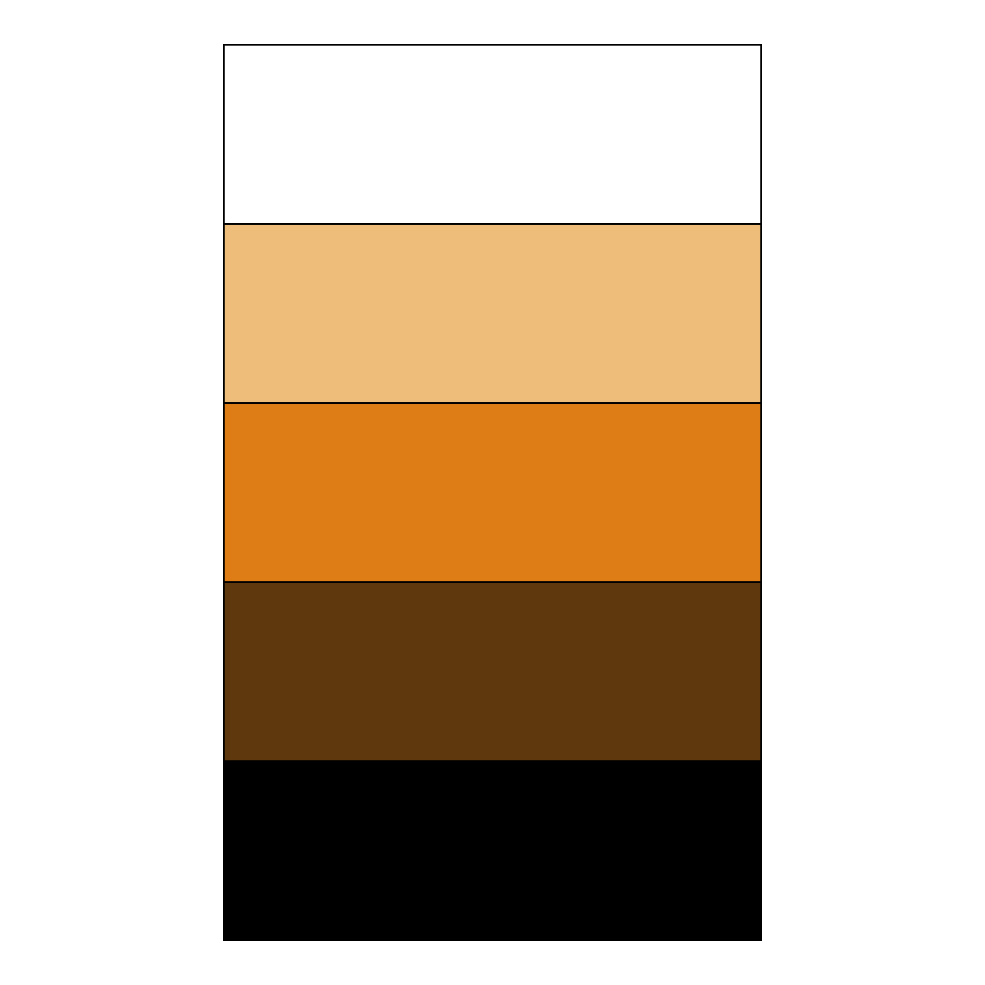
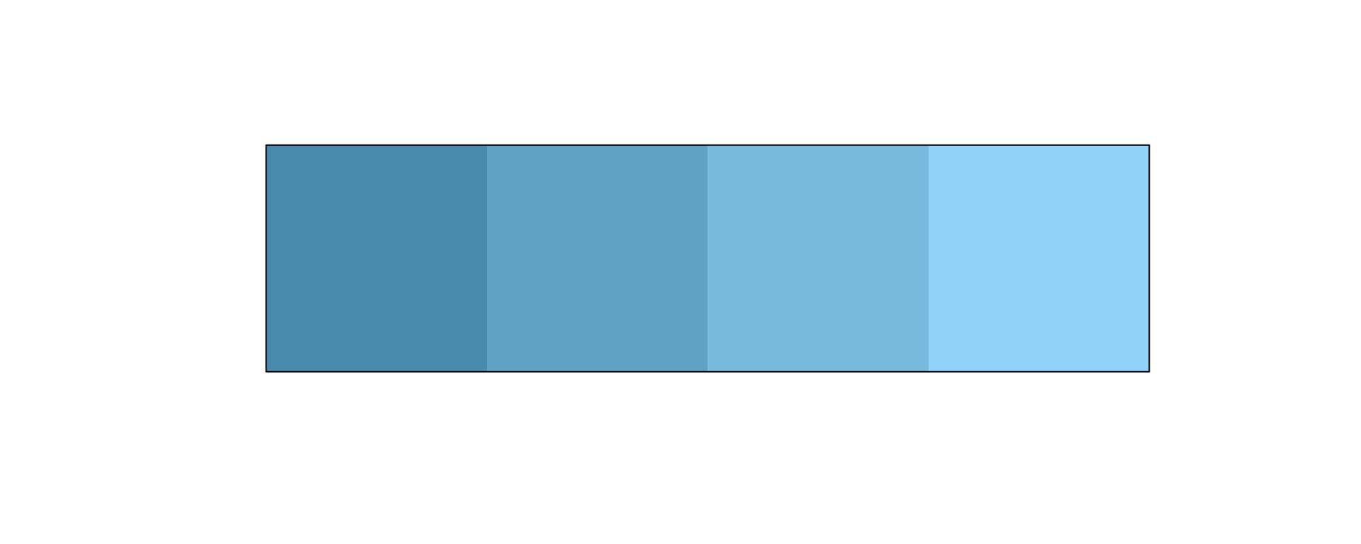
Monochromatic

Multiple tones of one color

Study for Homage to the Square, 1972

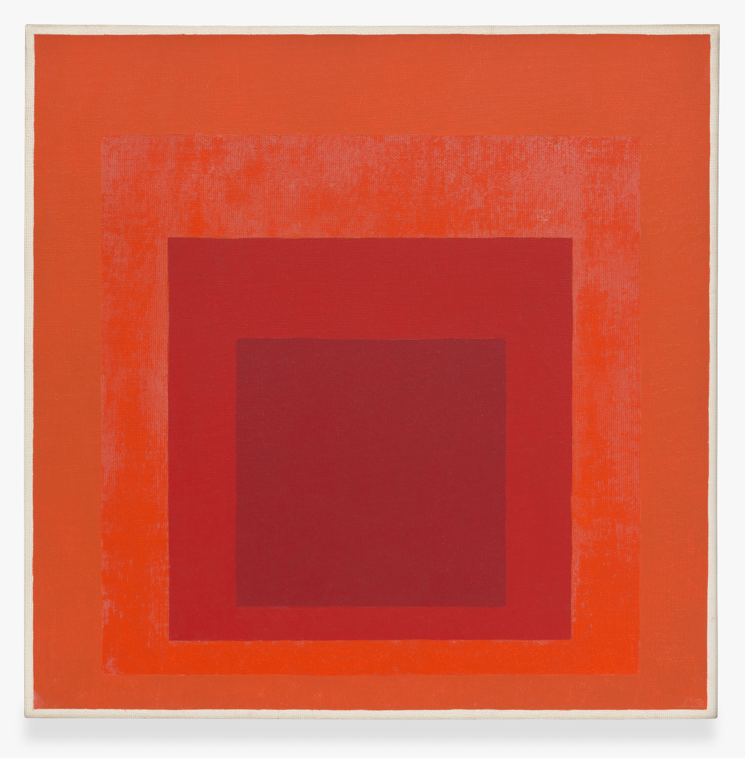
“If one says ‘red’ (the name of a color) and there are 50 people listening, it can be expected that there will be 50 reds in their minds. And one can be sure that all these reds will be very different.”

— Josef Albers, Interaction of Color (1963)

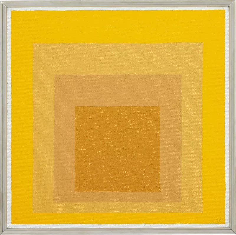
Study to Homage to the Square - Endless, 1964

Same yellow from different paint companies

Monochromatic

Provides a subtle and conservative color combination. This is a versatile color combination that is easy to apply to design projects for a harmonious look.

monochromatic <- tribble(
  ~color,
  mystery_color,
  mystery_color %>% 
    clr_lighten(shift = 0.20),
  mystery_color %>% 
    clr_lighten(shift = 0.40),
  mystery_color %>% 
    clr_lighten(shift = 0.60)
)

plot(monochromatic[["color"]])

make_homage(
  seed = 1,
  colors = monochromatic[["color"]]
)

Analogous

Three colors side by side on the color wheel

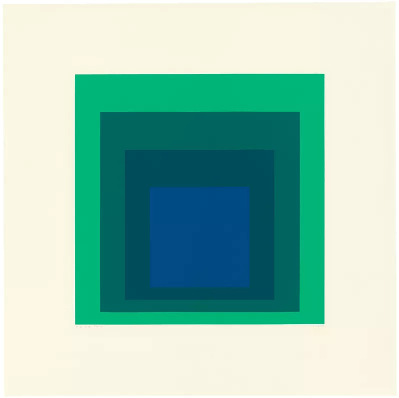
Homage to the Square: Edition Keller Ia, 1970

Analogous

This color combination is versatile, but can be overwhelming. To balance an analogous color scheme, choose one dominant color, and use the others as accents.

analogous <- tribble(
  ~color,
  mystery_color %>% 
    clr_lighten(shift = 0.20),
  mystery_color,
  mystery_color %>% 
    clr_rotate(degrees = 30),
  mystery_color %>% 
    clr_rotate(degrees = 60)
)

plot(analogous[["color"]])

make_homage(
  seed = 2,
  colors = analogous[["color"]]
)

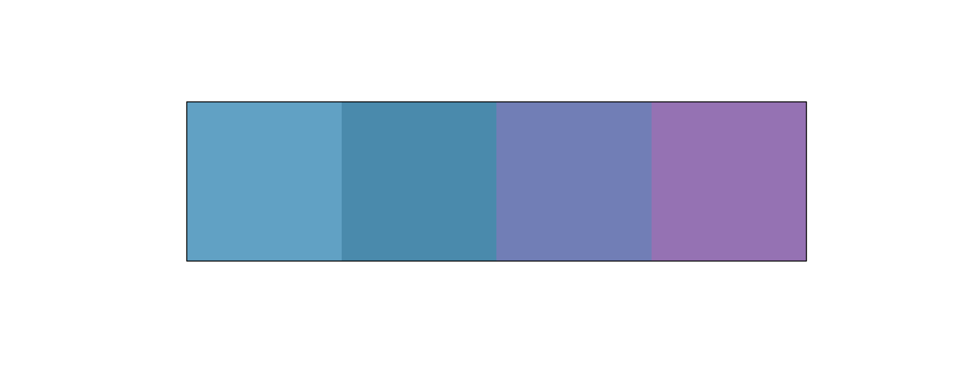
Analogous

That was a bit ugly - add contrast in other ways

analogous_better <- tribble(
  ~color,
  mystery_color %>% 
    clr_lighten(shift = 0.50),
  mystery_color,
  mystery_color %>% clr_rotate(degrees = 30) %>%
    clr_lighten(shift = 0.25),
  mystery_color %>% clr_rotate(degrees = 60) %>%
    clr_darken(shift = 0.25)
)

plot(analogous_better[["color"]])

make_homage(
  seed = 3,
  colors = analogous_better[["color"]]
)

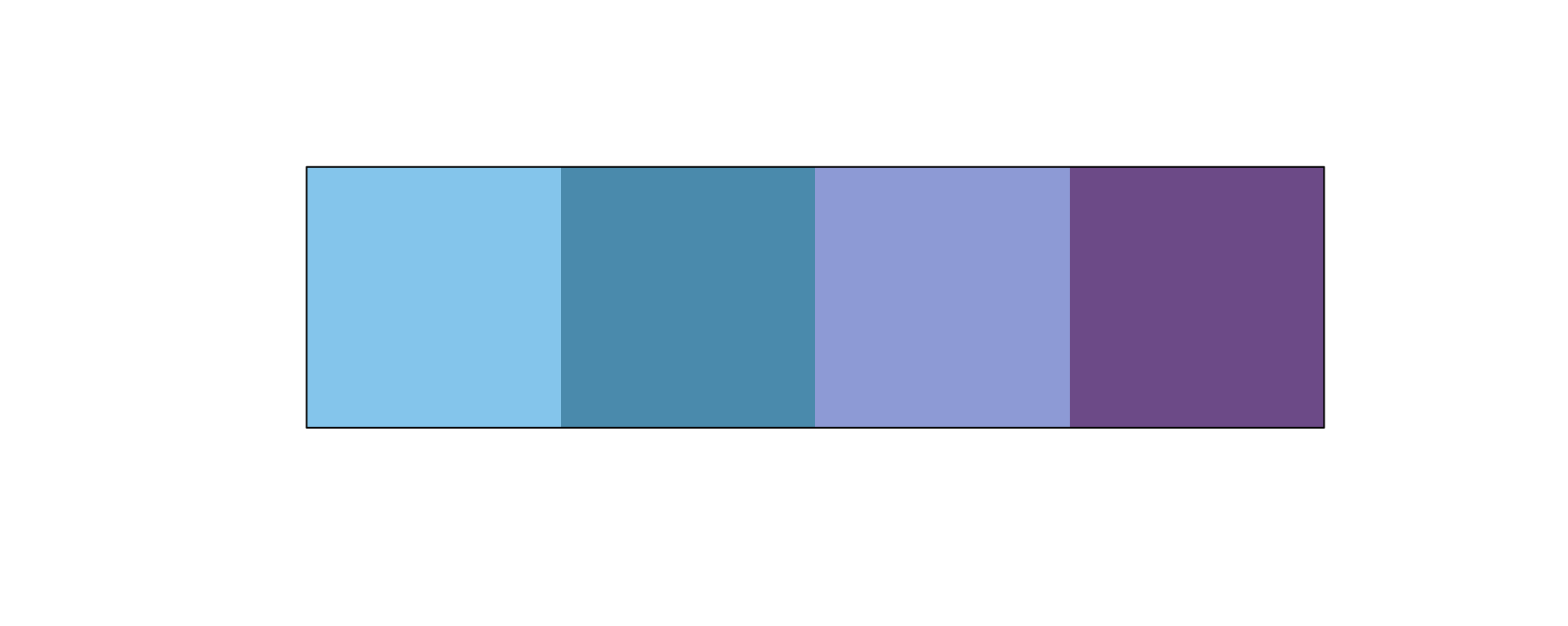
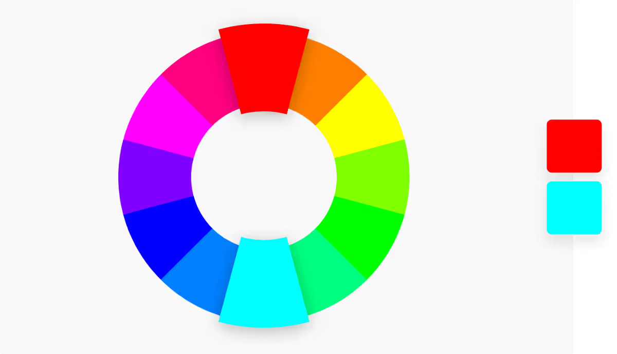
Complementary

This combination provides a high contrast and high impact color combination – together, these colors will appear brighter and more prominent.

Two colors on opposite sides of the color wheel

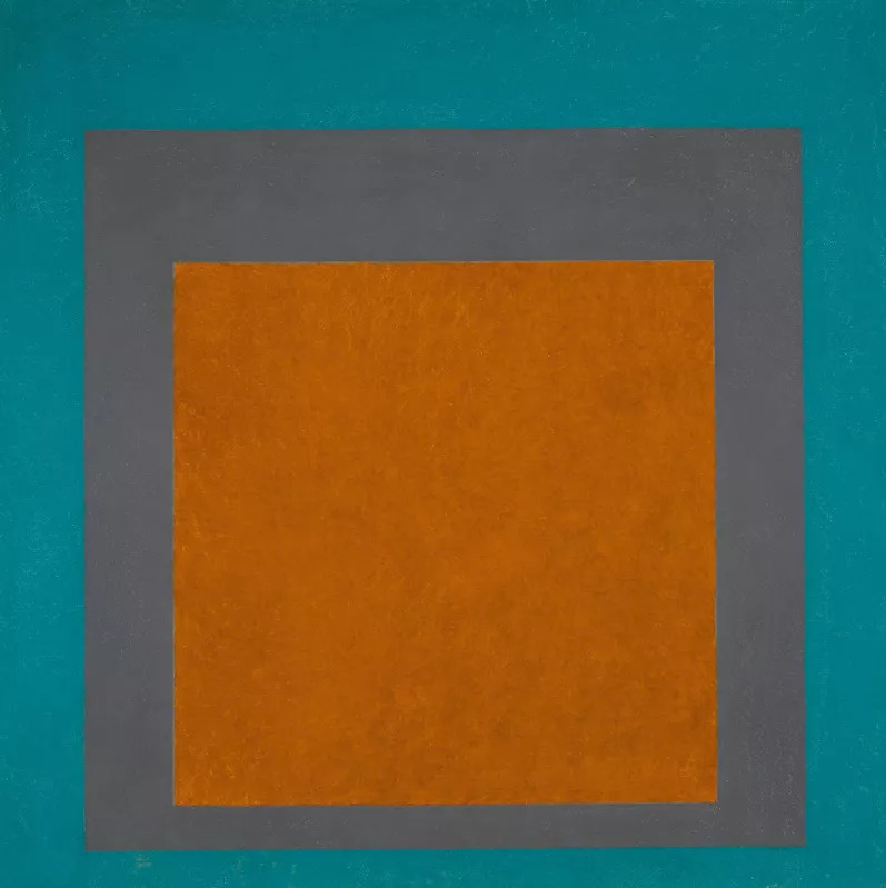
Homage to the Square: Earth and Air, 1965

Complementary

monochromatic_mini <- tribble(
  ~color,
  mystery_color %>% clr_lighten(shift = 0.20),
  mystery_color
)
complementary <- bind_rows(
  monochromatic_mini,
  monochromatic_mini %>%
    mutate(
      color = clr_rotate(color,
        degrees = 360 / 2
      )
    )
)
plot(complementary[["color"]])

make_homage(
  seed = 3,
  colors = complementary[["color"]]
)

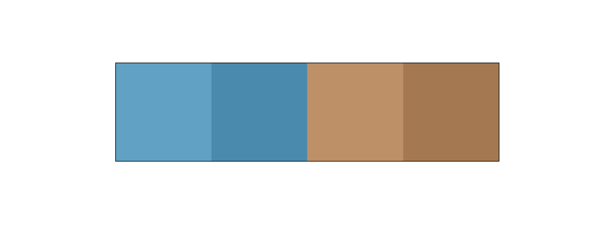
Complementary

Having the same saturation and lightness doesn’t always work!

monochromatic_mini <- tribble(
  ~color,
  mystery_color %>%
    clr_lighten(shift = 0.75),
  mystery_color
)

complementary <- bind_rows(
  monochromatic_mini,
  monochromatic_mini %>%
    mutate(
      color = clr_rotate(color,
        degrees = 360 / 2
      ),
      color = clr_desaturate(color,
        shift = 0.5
      )
    )
)

plot(complementary[["color"]])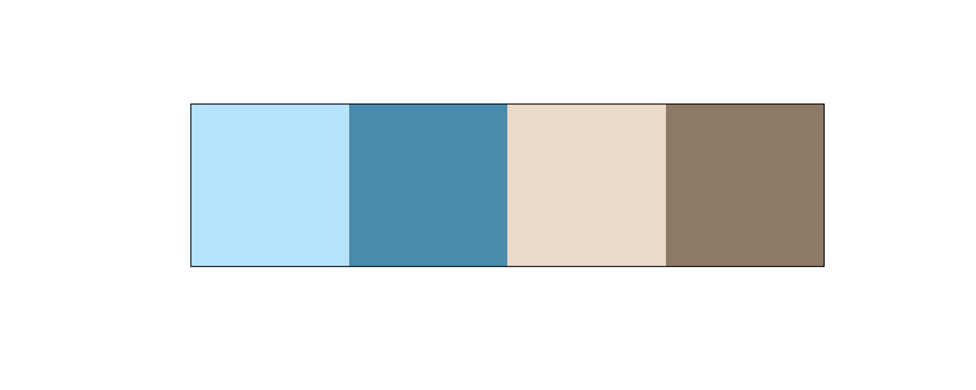

Complementary

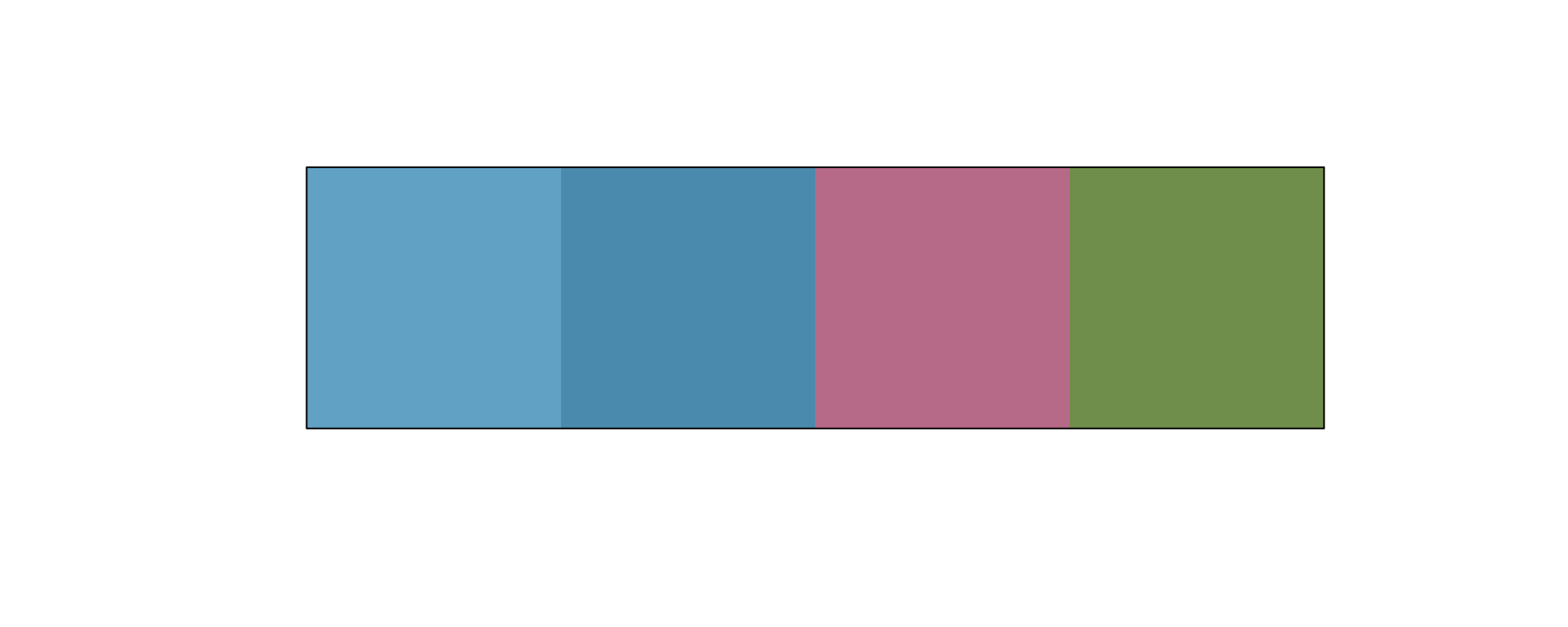
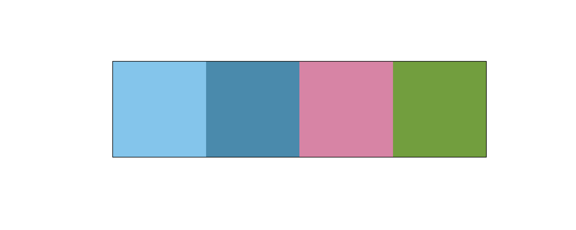
Having the same saturation and lightness doesn’t always work!

make_homage(
  seed = 3,
  colors = complementary[["color"]]
)

Complementary

This is the hue of the colors of our original piece - not exactly opposite on the color wheel, but very close!

Triadic

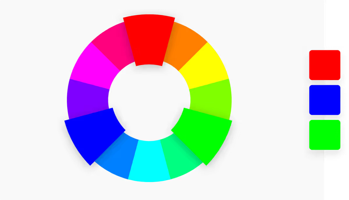
Three colors evenly spaced on the color wheel

This provides a high contrast color scheme, but less so than the complementary color combination — making it more versatile. This combination creates bold, vibrant color palettes.

Triadic

triadic <- tribble(
  ~color,
  mystery_color %>% 
    clr_lighten(shift = 0.20),
  mystery_color,
  mystery_color %>%
    clr_rotate(degrees = 360 / 3),
  mystery_color %>%
    clr_rotate(degrees = 2 * 360 / 3)
)

plot(triadic[["color"]])

make_homage(
  seed = 5,
  colors = triadic[["color"]]
)

Triadic

triadic <- tribble(
  ~color,
  mystery_color %>% 
    clr_lighten(shift = 0.50),
  mystery_color,
  mystery_color %>%
    clr_rotate(degrees = 360 / 3) %>%
    clr_lighten(0.25),
  mystery_color %>%
    clr_rotate(degrees = 2 * 360 / 3) %>%
    clr_saturate(0.15)
)

plot(triadic[["color"]])

make_homage(
  seed = 5,
  colors = triadic[["color"]]
)

Cool and warm colors

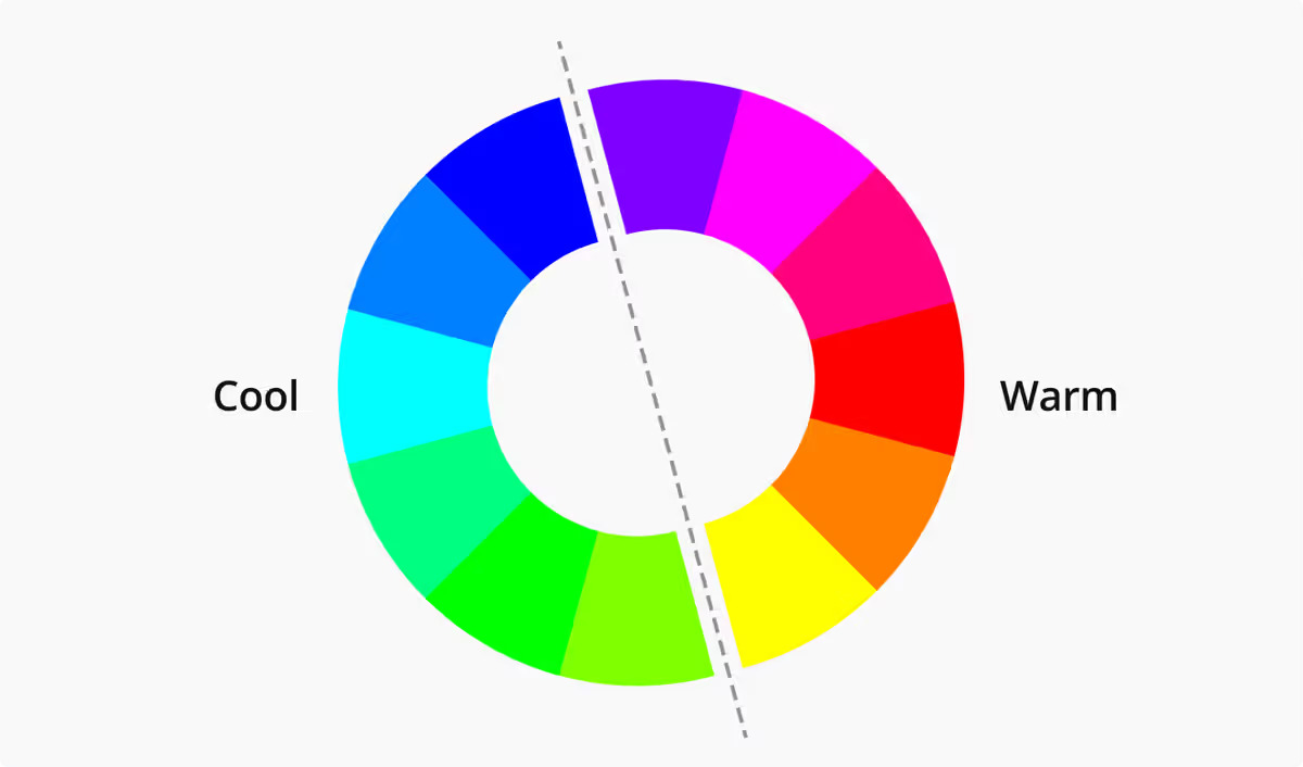
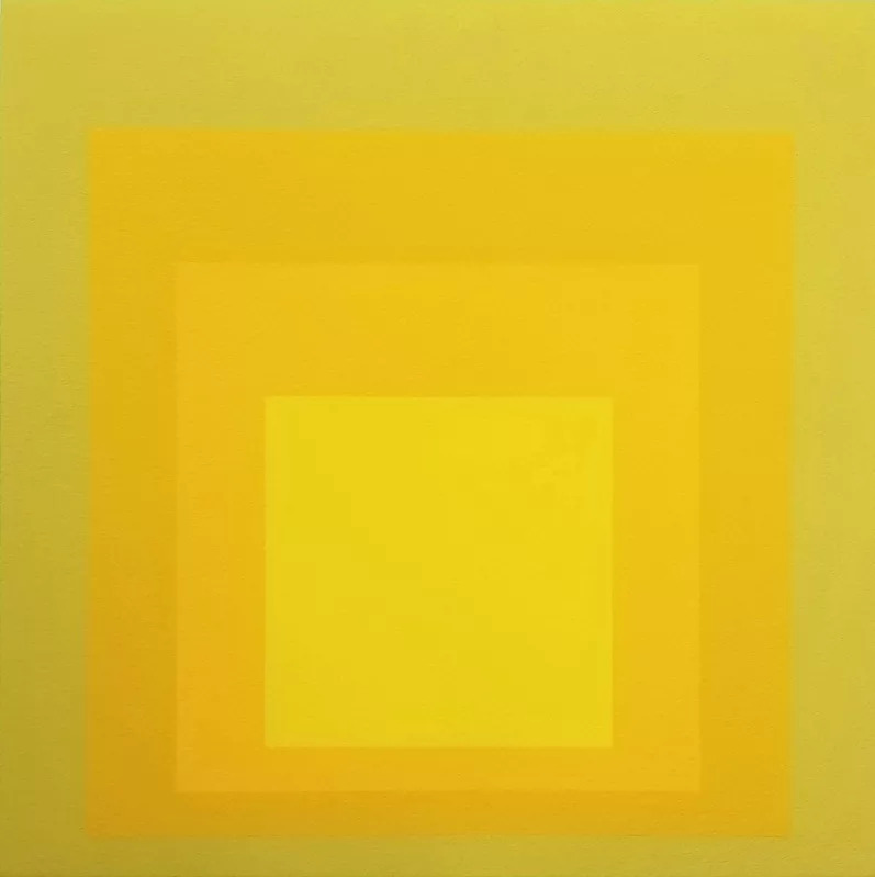
EK Ic, 1970

Finding palettes

What inspires you?

IKEA, 1984

Studio GdB

@hyunakimberly

Luna Wear

My Bloody Valentine

Hannah Stahl

Can Yang

IKEA, 1984

Furniture, art, clothing, music, movies, nature, books

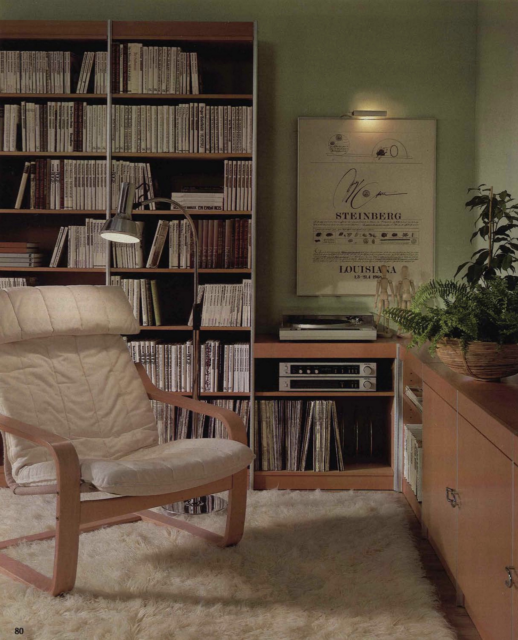
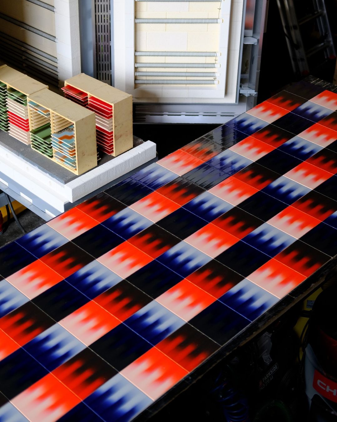
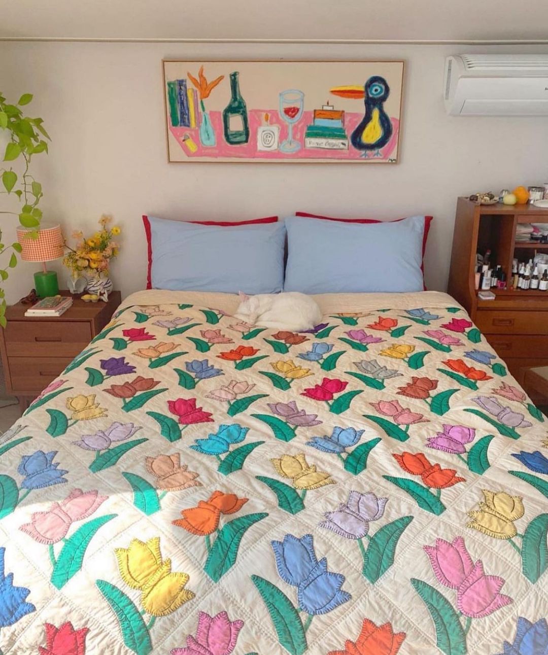
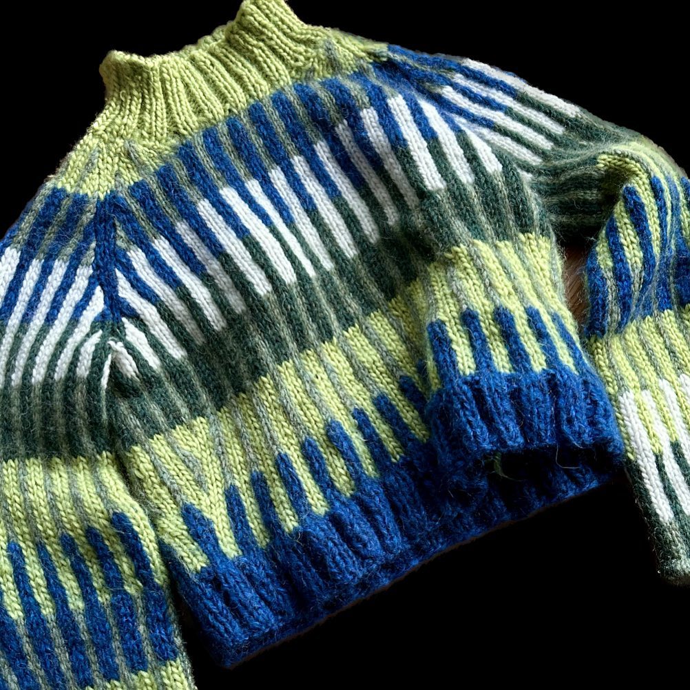
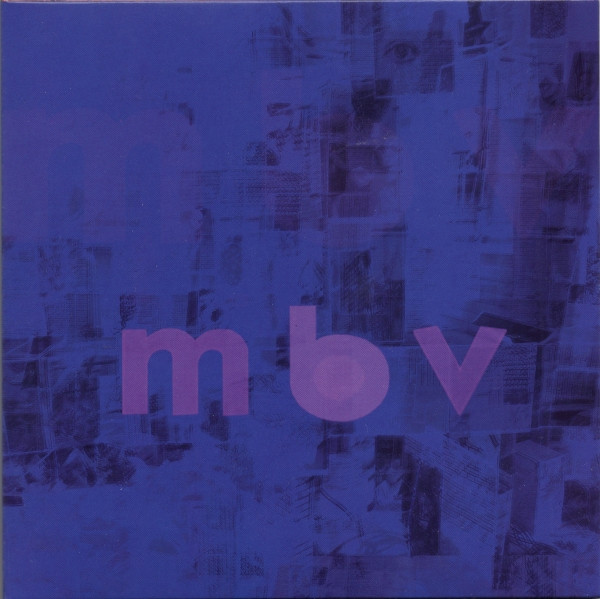
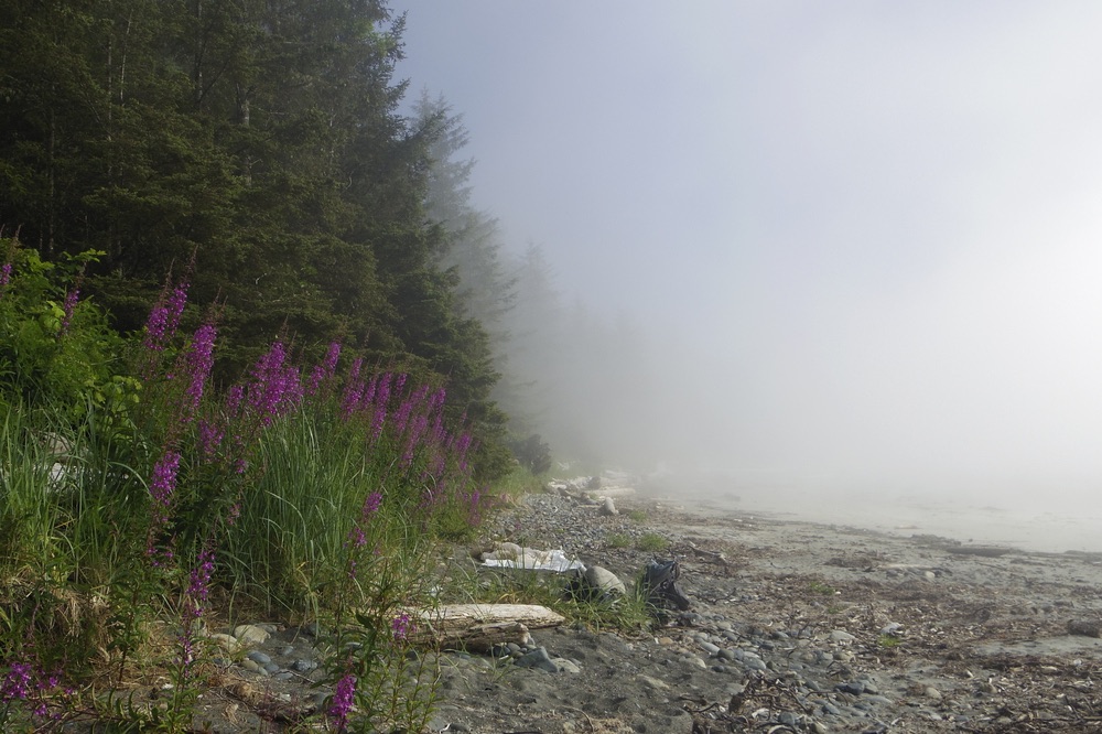
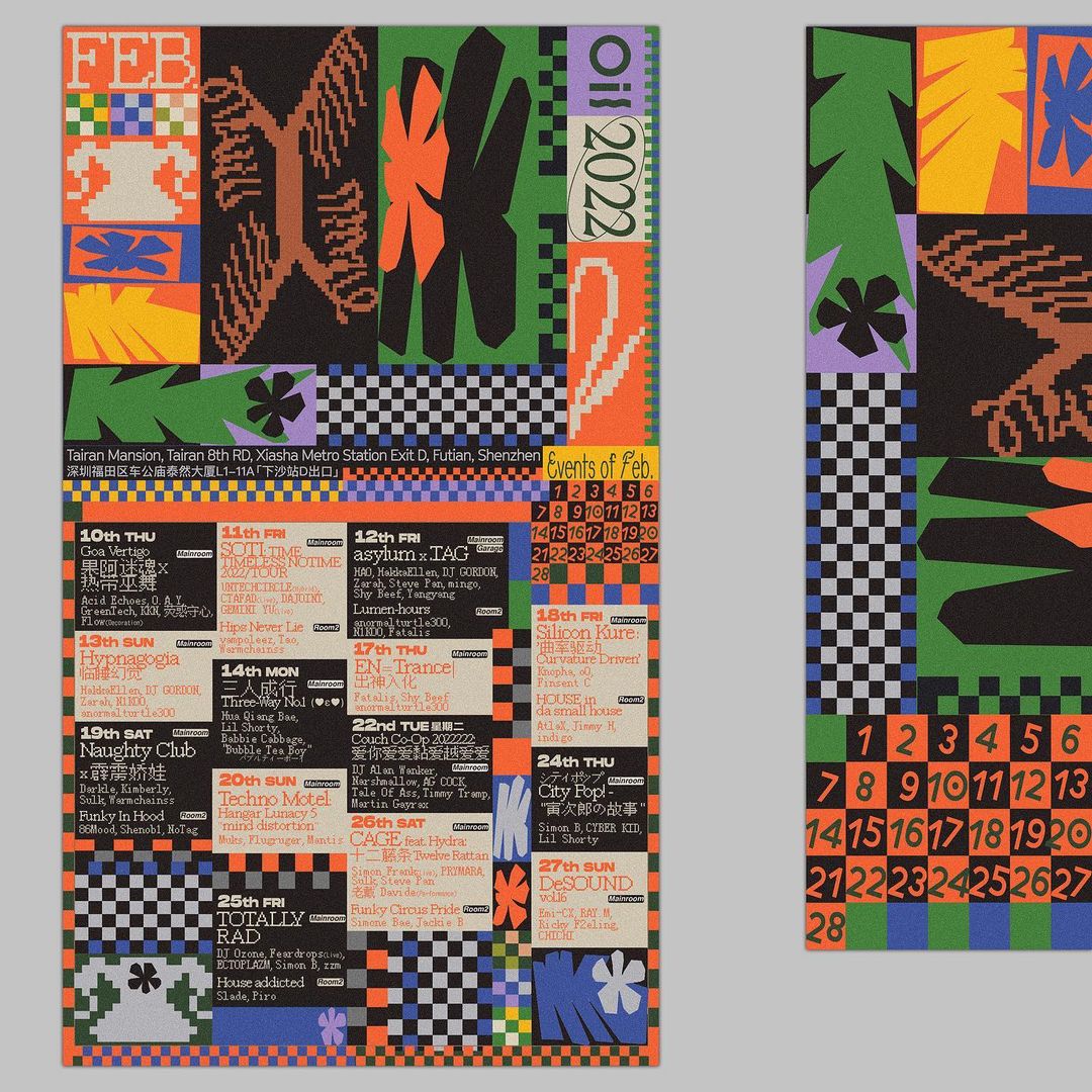
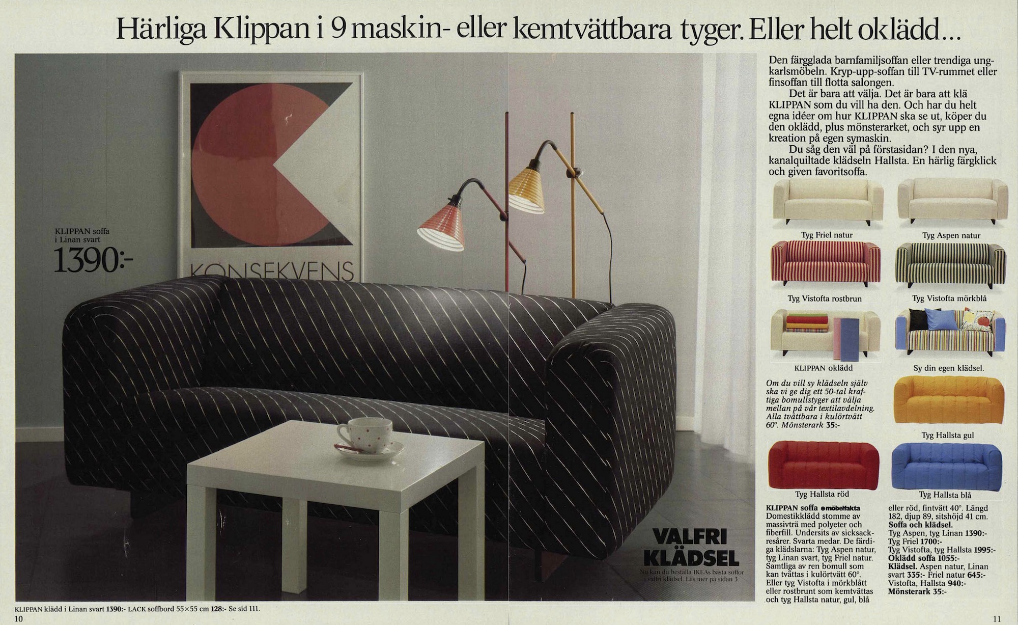
What inspires you?

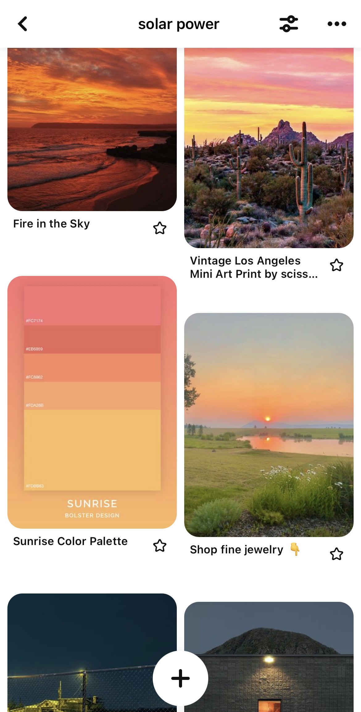
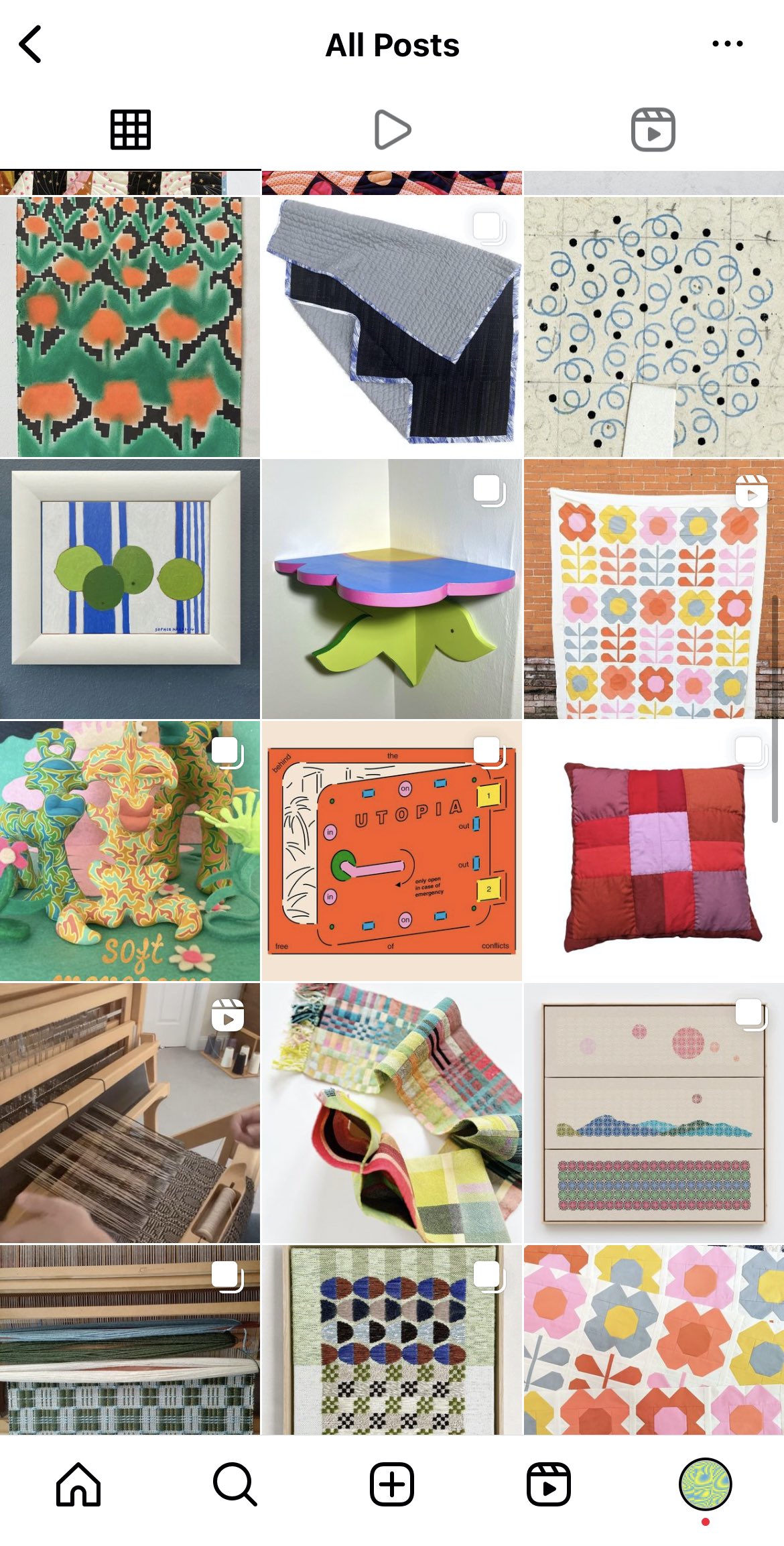
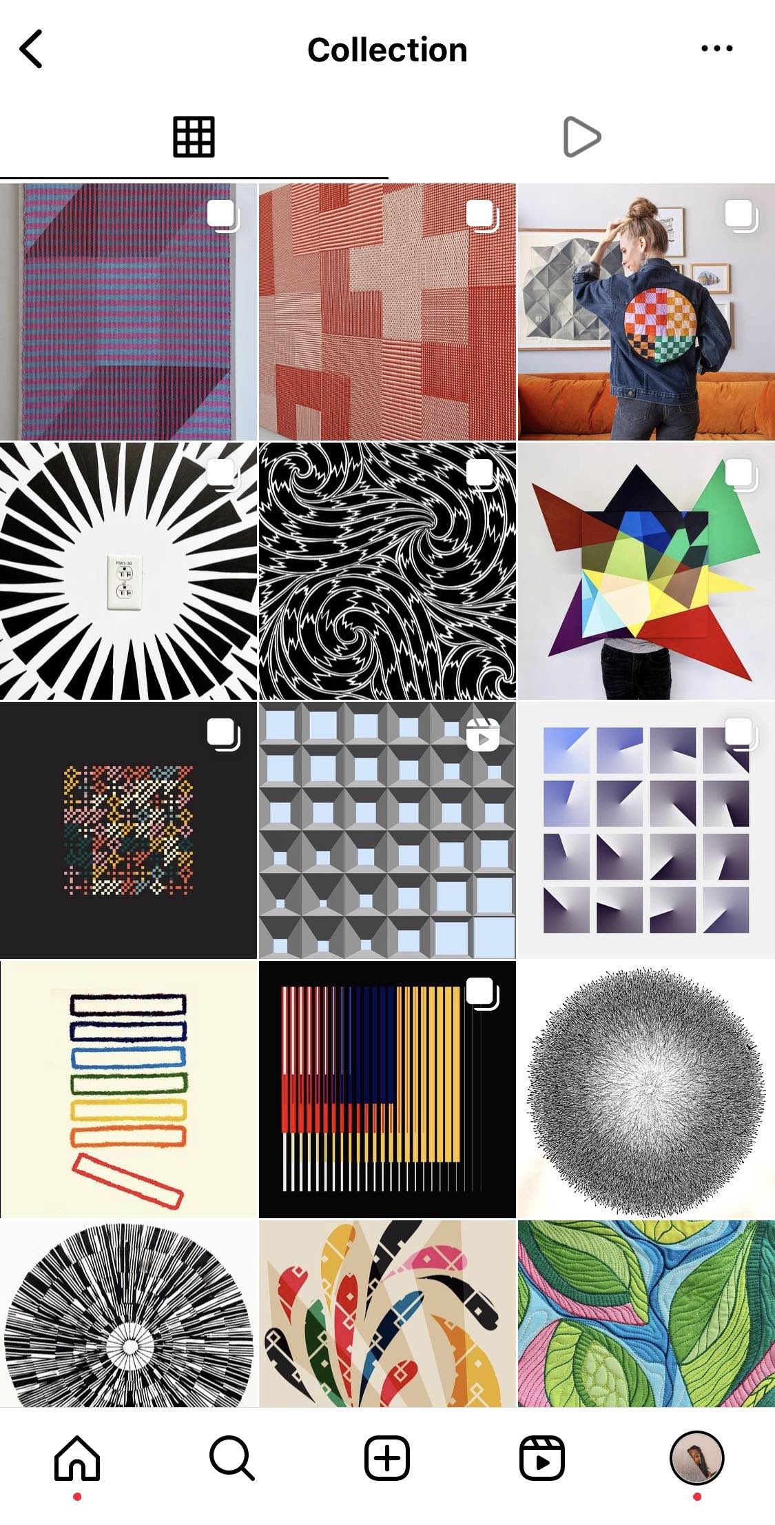
When in doubt, steal

Show upload and link, good time to show system in R and paste colors in

ColorGrab

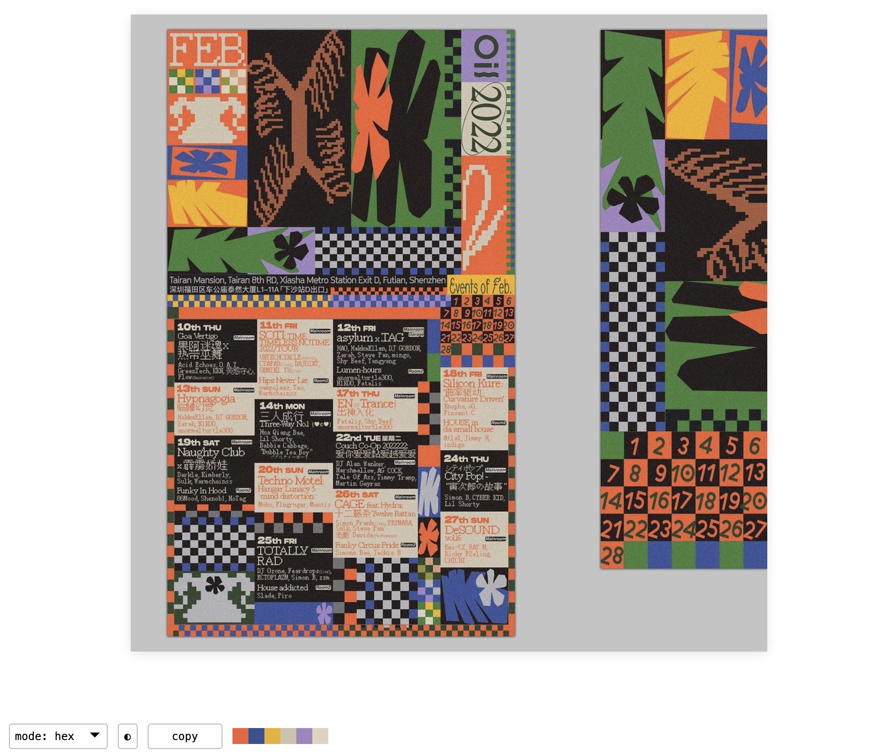
Some concrete sources

• Google Arts & Culture: Art Palette
• Colours Cafe
• Coolors palette generator
• color-hex
• ColorSpace

Remix

1. Open the file exercises/02-homage-to-the-square/exercise-2.Rmd
2. Find an inspiration image and extract colors, or choose a palette from one of the sources above. Make sure you have at least 4 colors!
3. Update the function make_my_homage() to take your palette as the default value of the colors argument
4. Run the function make_my_homage() with a few different seeds and pick your output
5. Share the inspiration and output in the GitHub discussion for this exercise

10:00

Inspired by Homage to the Square

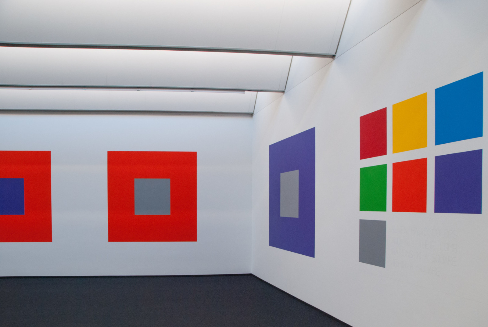
Seven Basic Colors and All Their Combinations in a Square within a Square: Wall Drawing for Josef Albers (Wall Drawing 1176), Sol LeWitt

Reinterpet

1. Take a few minutes to imagine what kind of work you could create inspired by Homage to the Square
2. Use whatever tool you like - paper, ggplot2, figma, anything you’re comfortable with!
3. Share your work in the GitHub discussion for this exercise

10:00

So far you’ve…

• Learned how to recreate an Homage to the square using geom_rect()
• Saved work in a good size/resolution using ggsave()
• Created your first generative art system and using set.seed() to control randomness
• Explored HSL as a color system, and learned how to alter colors using their saturation and lightness
• Learned different methods of choosing cohesive color palettes color: monochromatic, analogous, complementary, triadic
• Found color inspiration and added your personal color touches to the Homages
• Imagined what other work you can create using rectangles and color

Break during break pls