Steal like an Rtist: Creative Coding in R
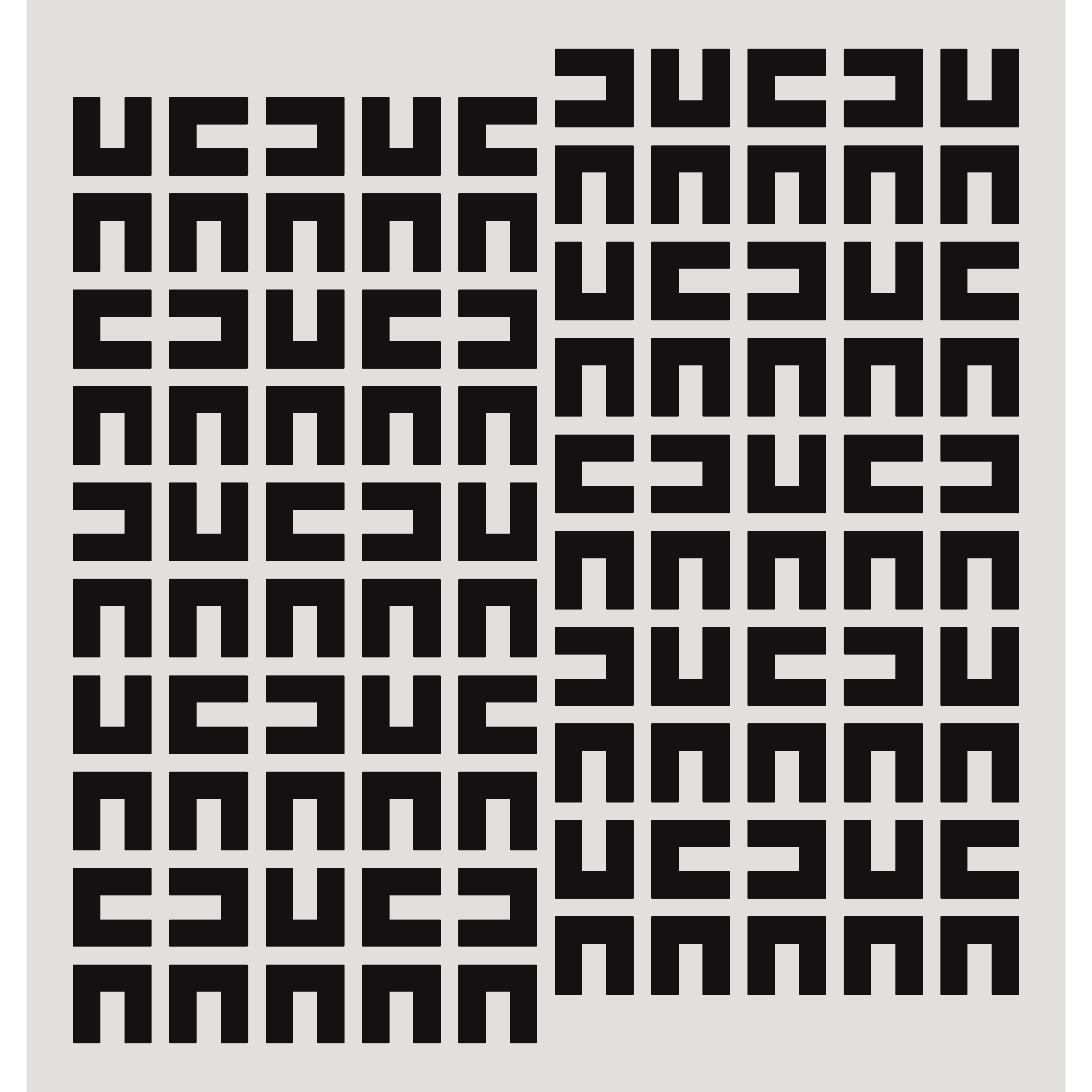
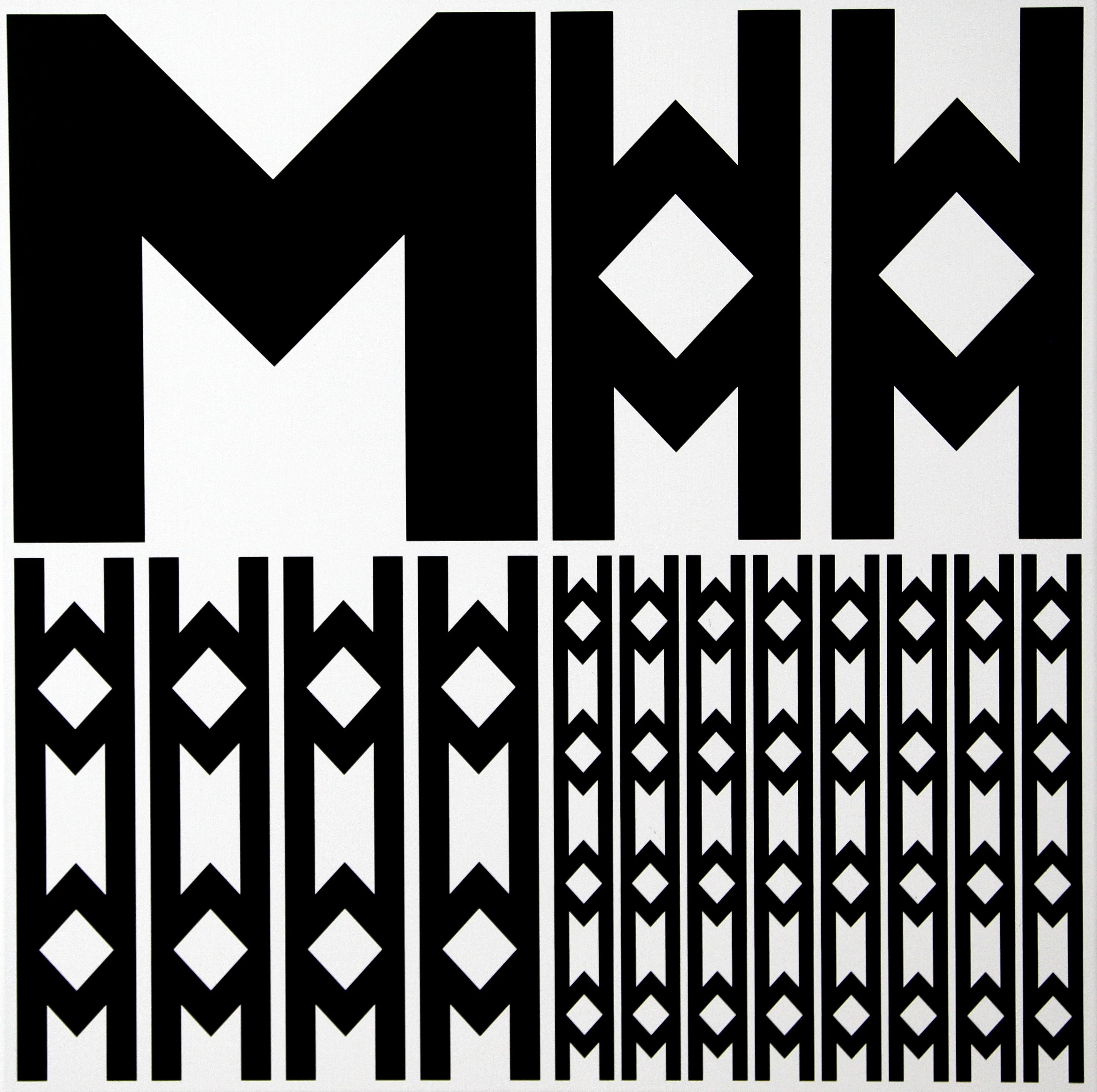
o.T. (carré noir)
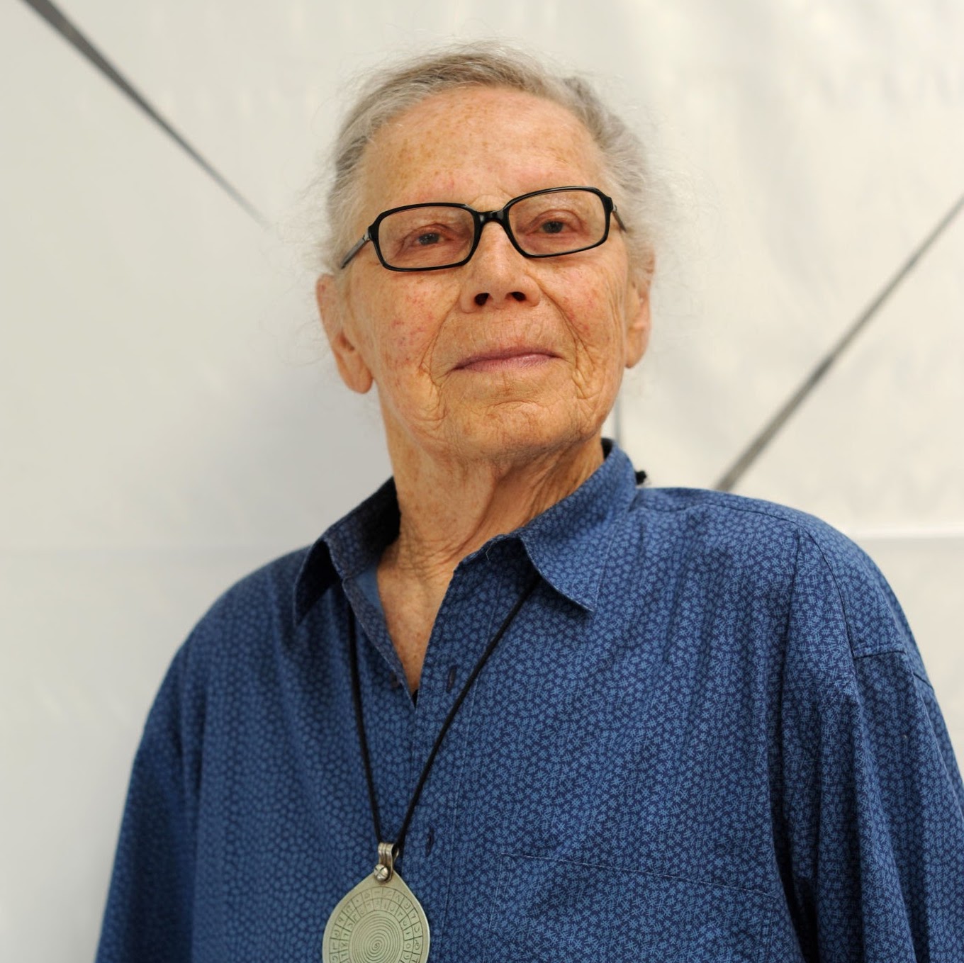
Vera Molnár
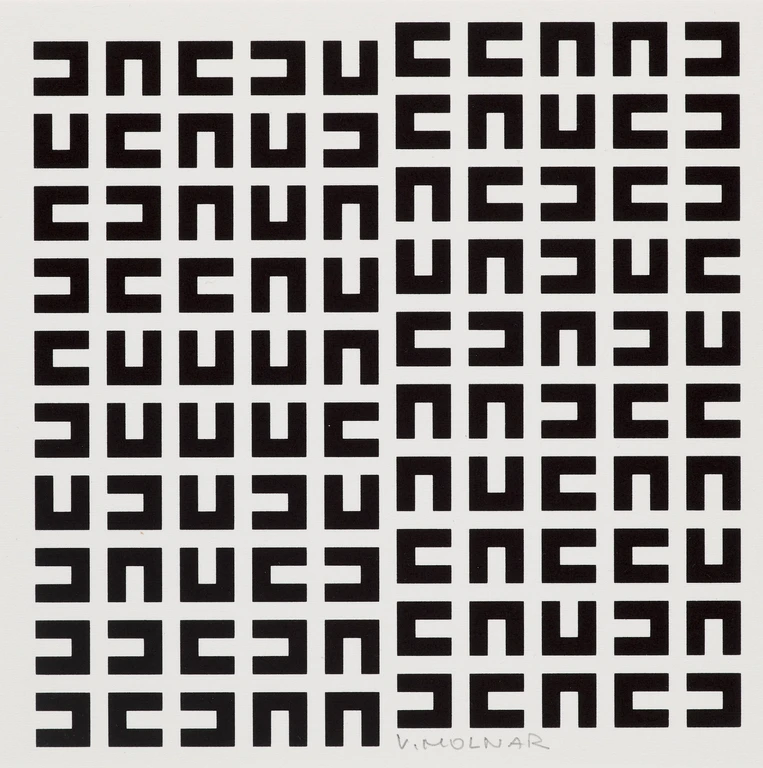
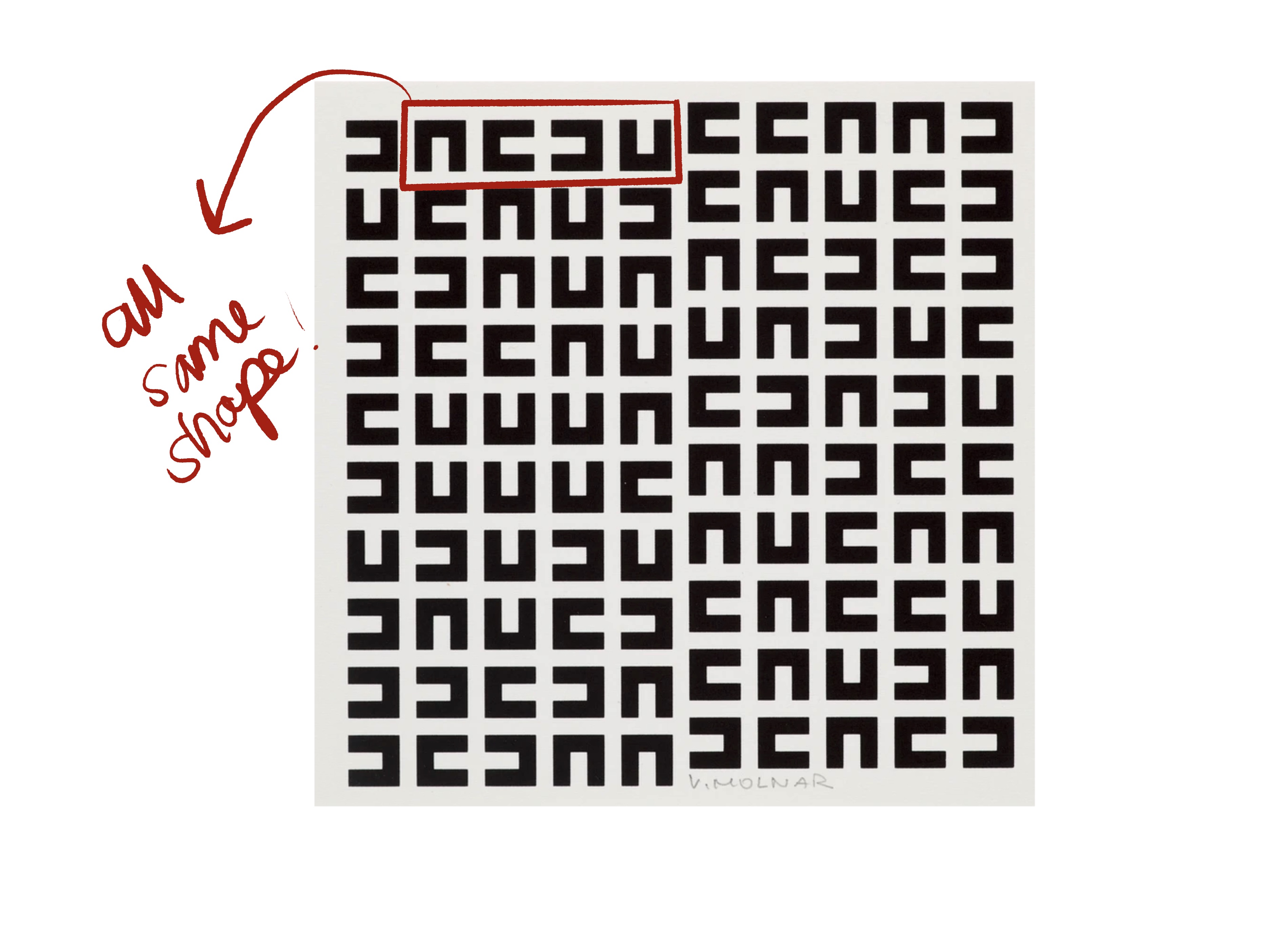
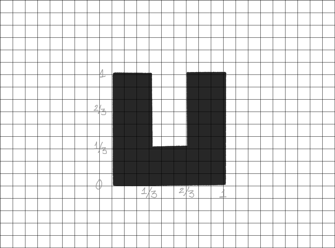
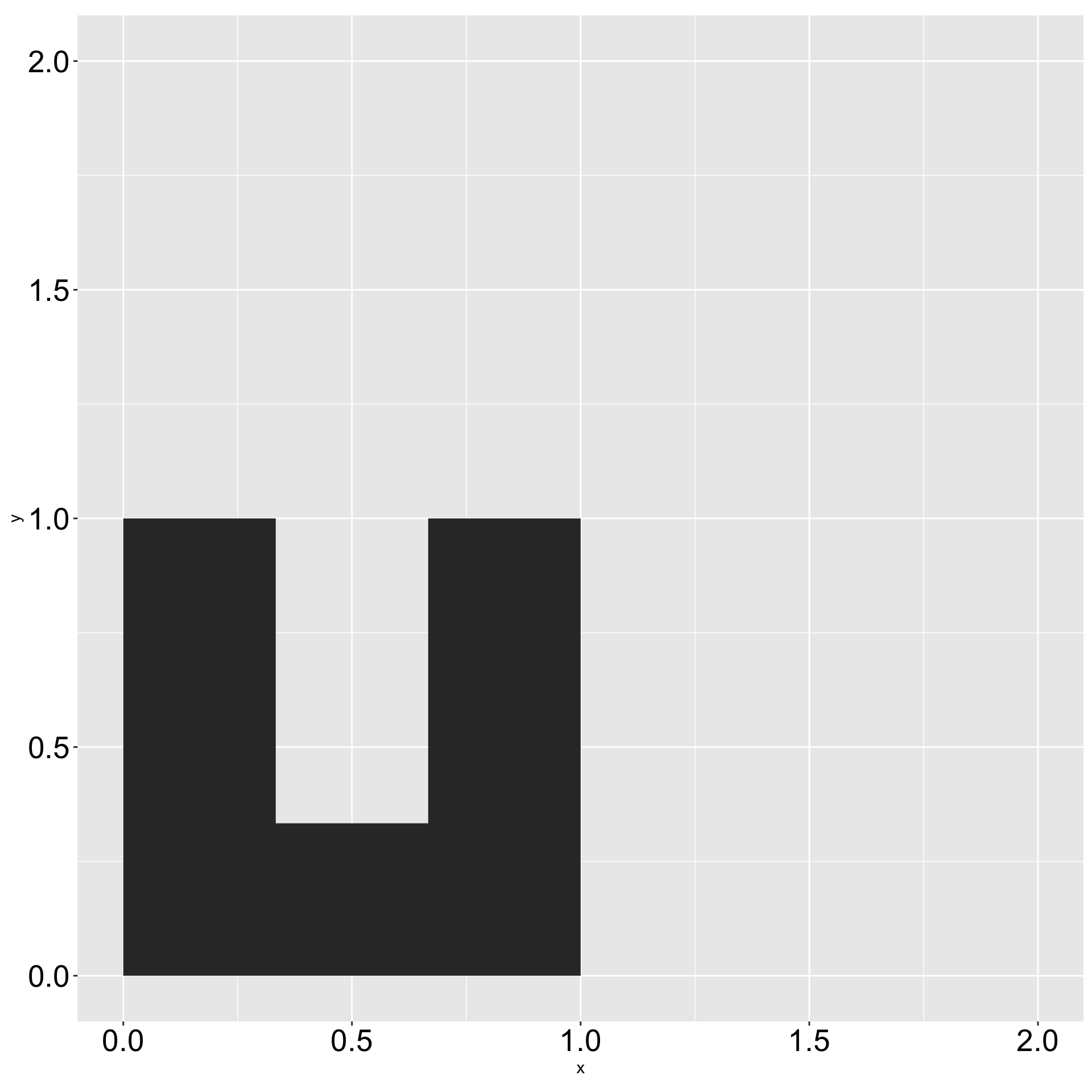
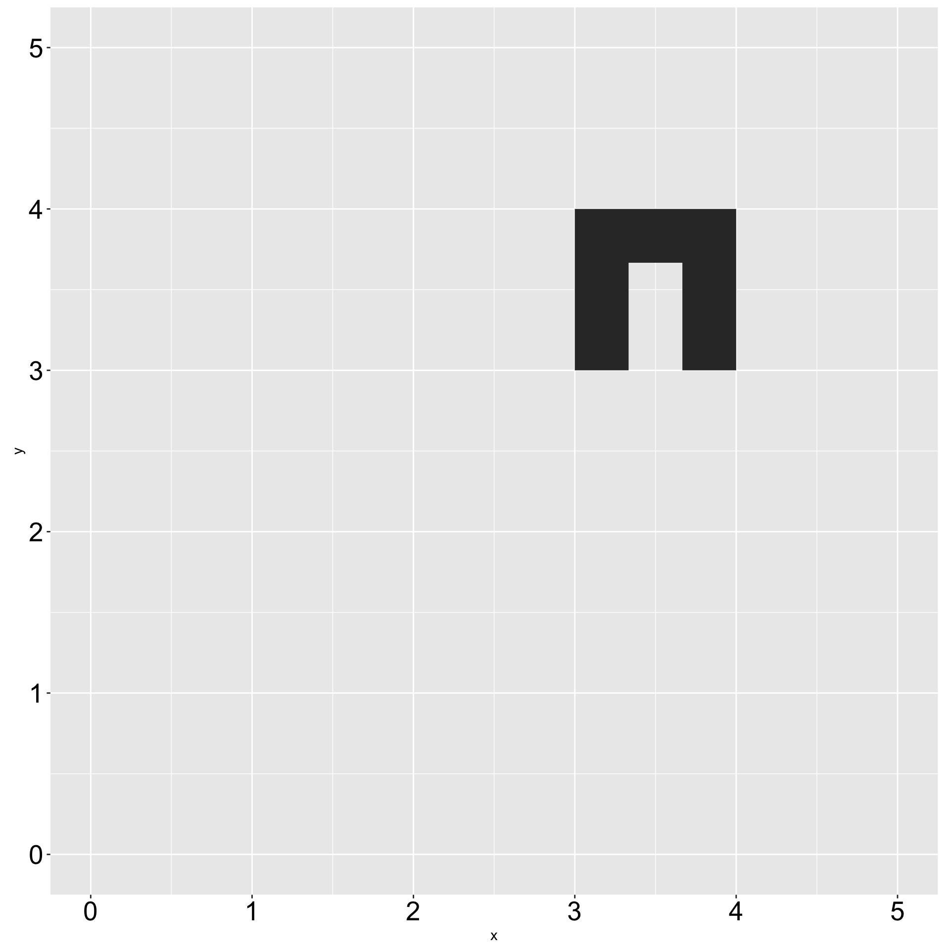
o.T. (carré noir): introduction to the shape
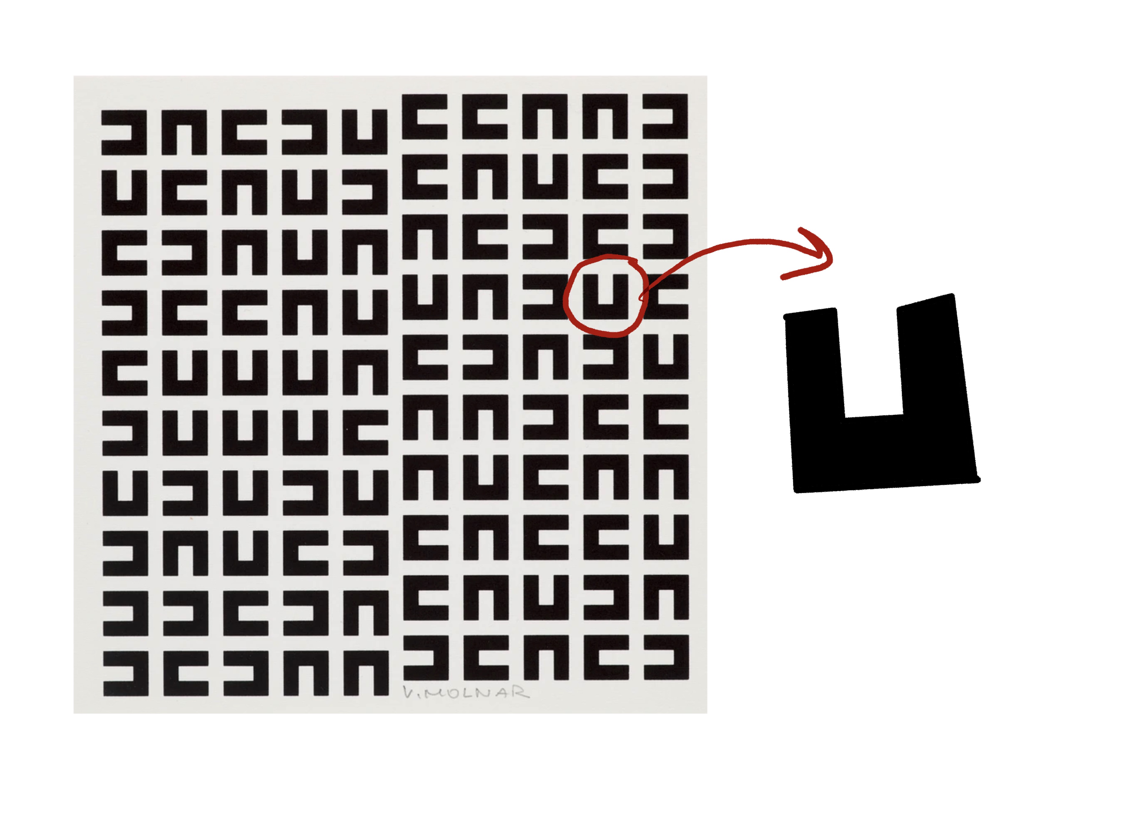
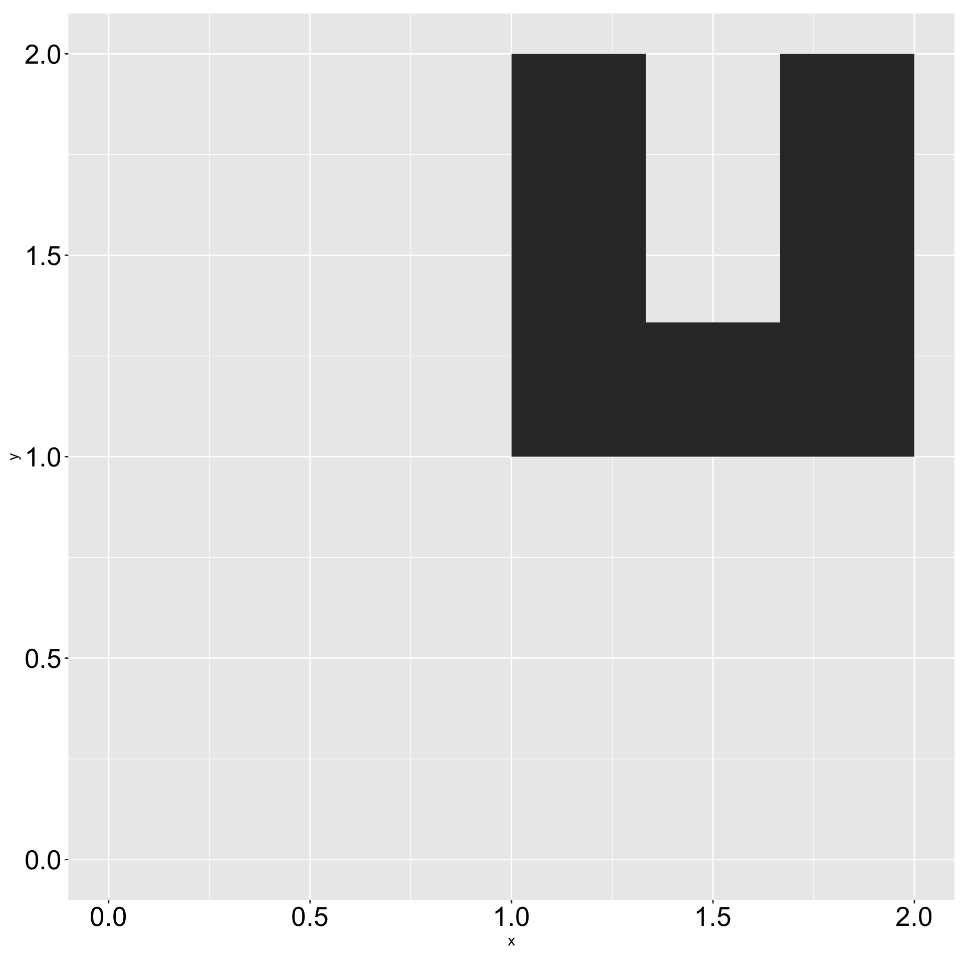
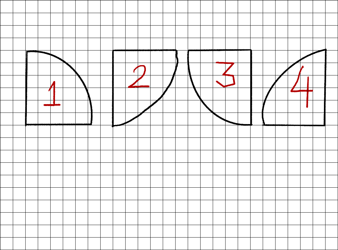
Orientation of the letter u
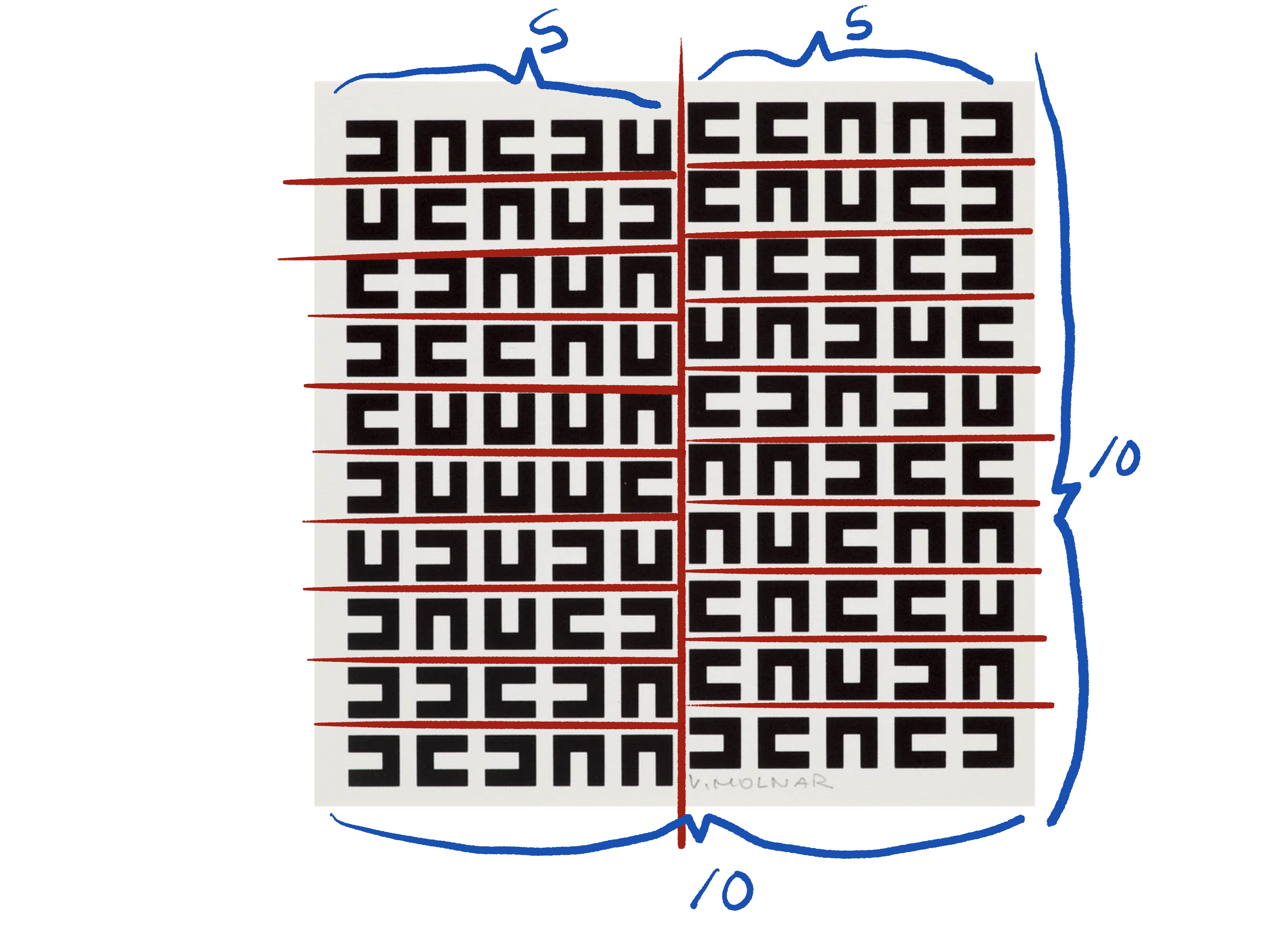
Composition of o.T. (carré noir)
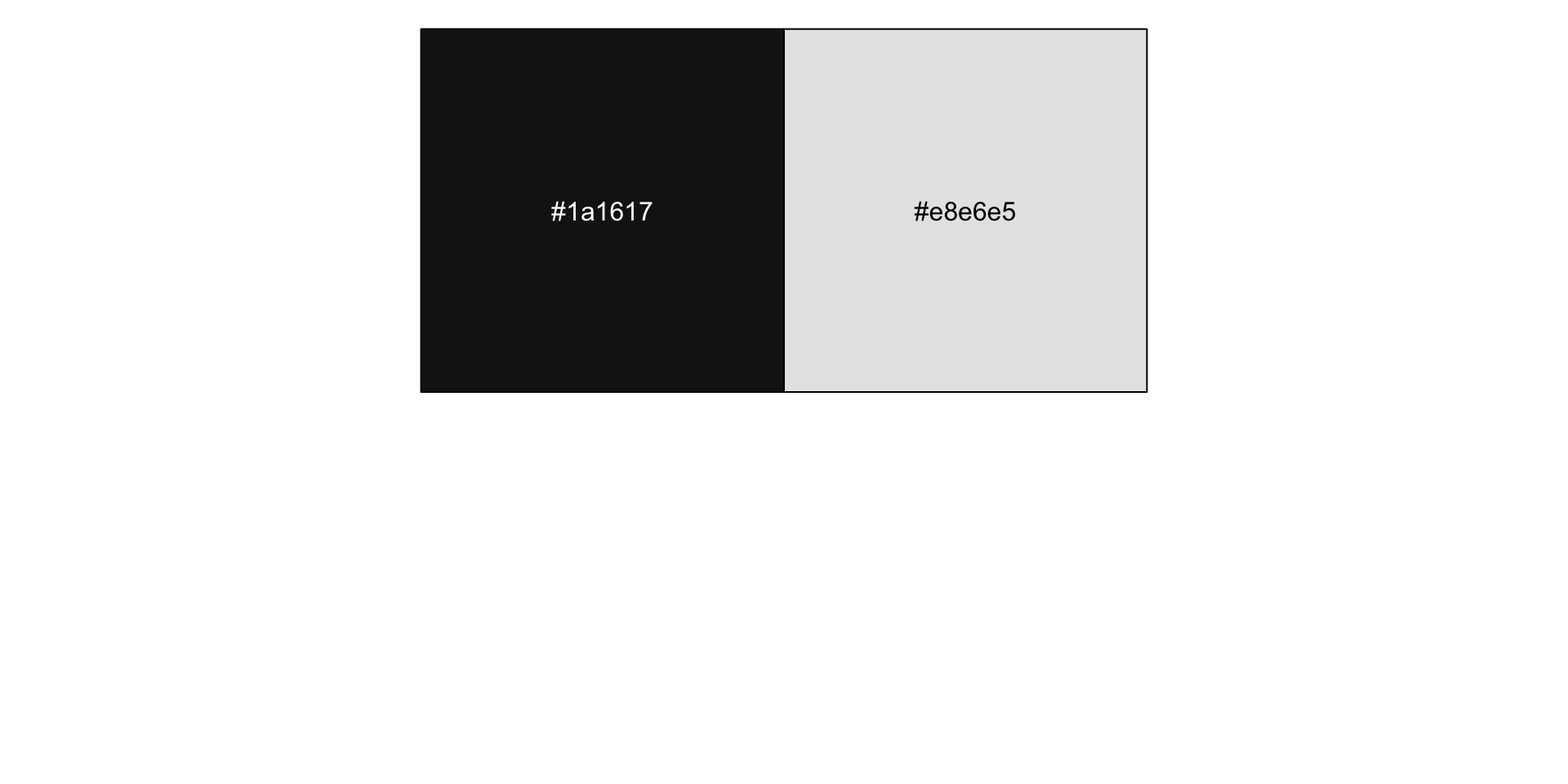
Color palette
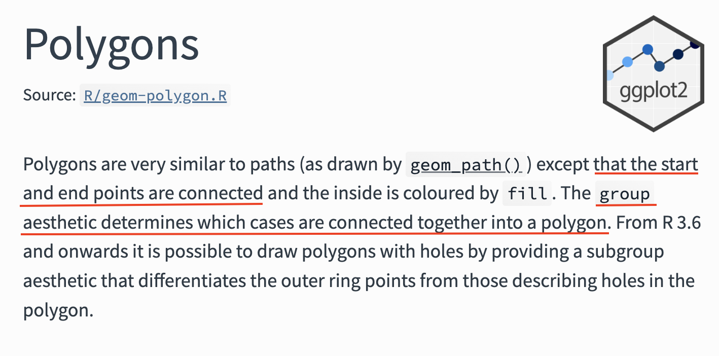
Creating polygons in {ggplot2}
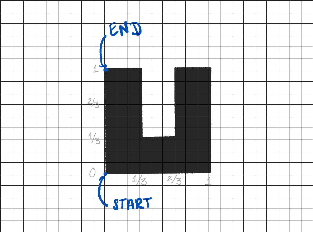
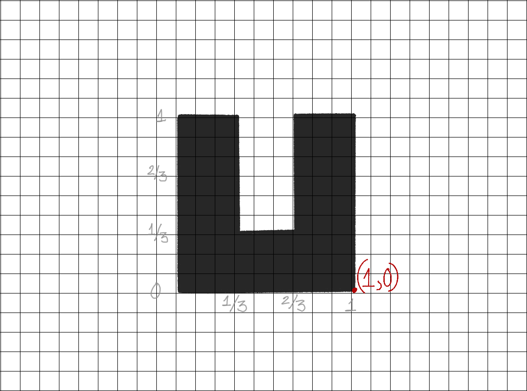
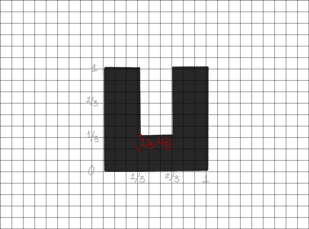
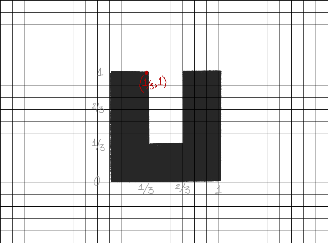
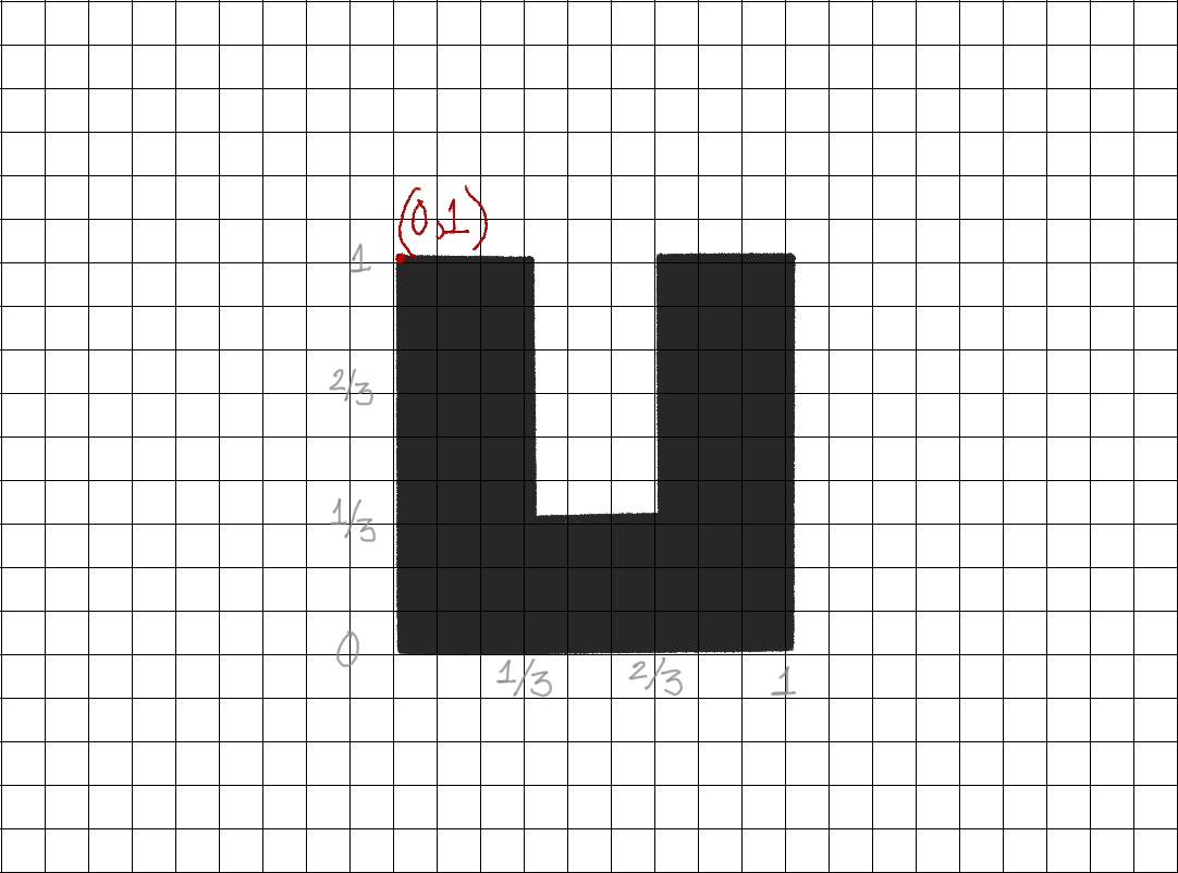
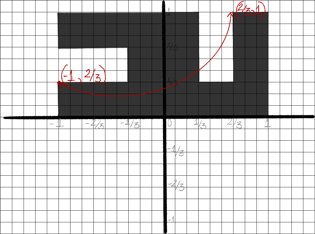
Coordinates of Letter U
Coordinates of Letter U
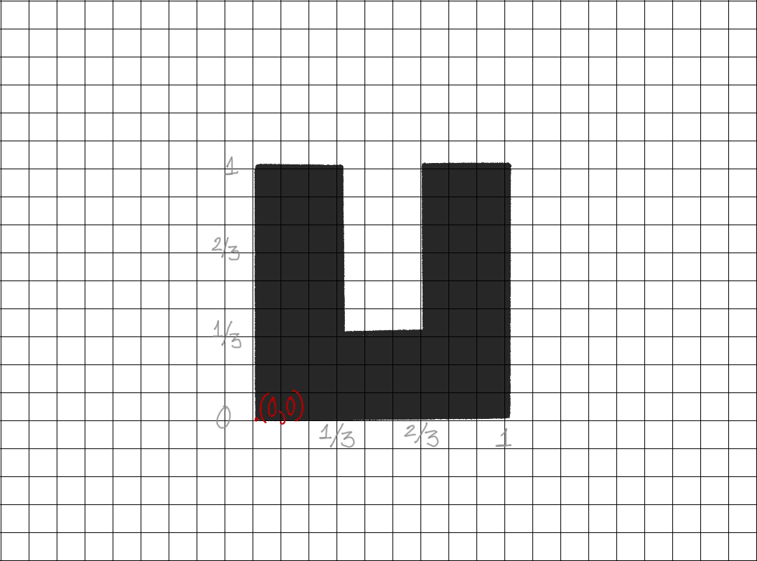
Go counterclockwise, starting from bottom left
Coordinates of Letter U
Only need coordinates from vertices in the polygon
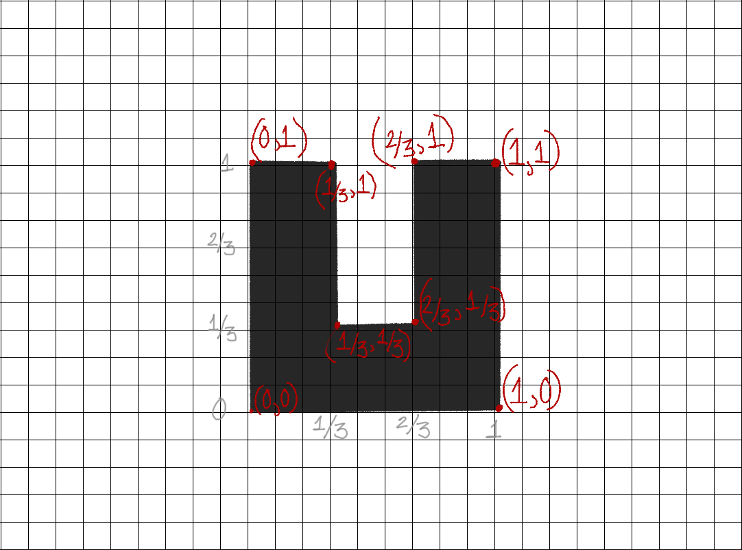
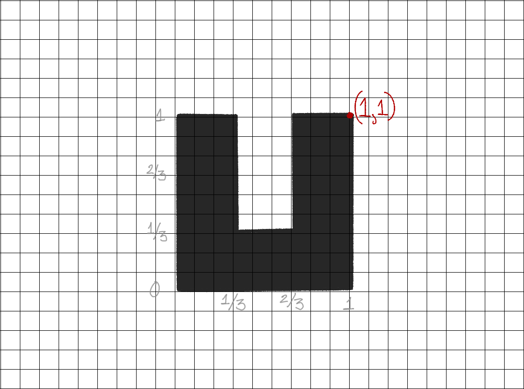
Coordinates of Letter U
Coordinates of Letter U
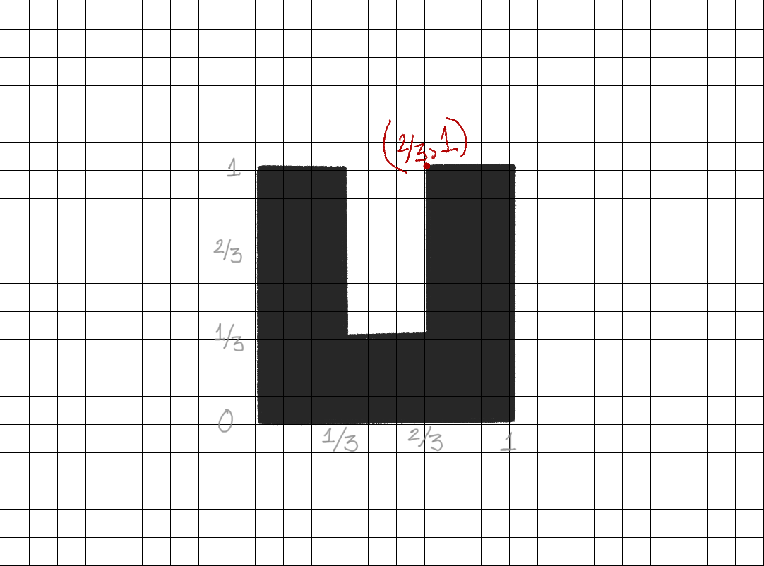
Coordinates of Letter U
Coordinates of Letter U
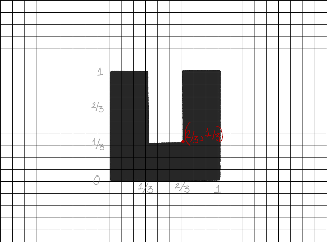
Coordinates of Letter U
Coordinates of Letter U
Coordinates of Letter U
Coordinates of Letter U
Coordinates of Letter U
Plotting Letter U
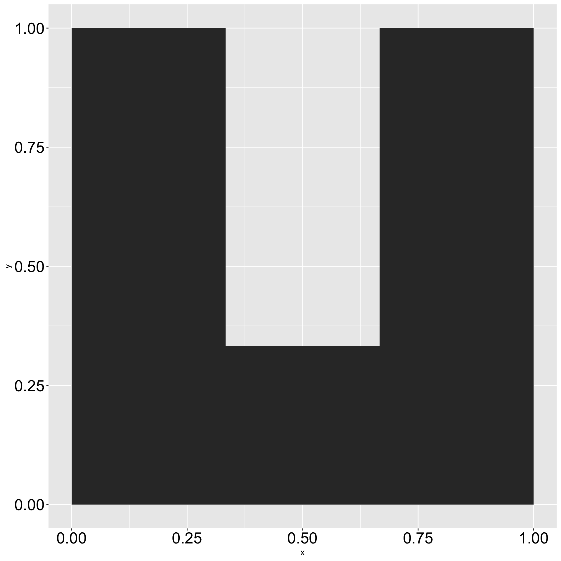
Plotting Letter U
Plotting Letter U
Adding flexibility

Plotting Letter U
Adding flexibility
Exploring Geometric Abstraction
“My life is in squares, triangles, lines”
Throughout her career, Vera Molnár experimented with repetitions and variations of letters, especially the letter M – as in Molnár.
She explored the balance between order and chaos.
A light trigonometry intermission
y_new = -x_old & x_new = y_old
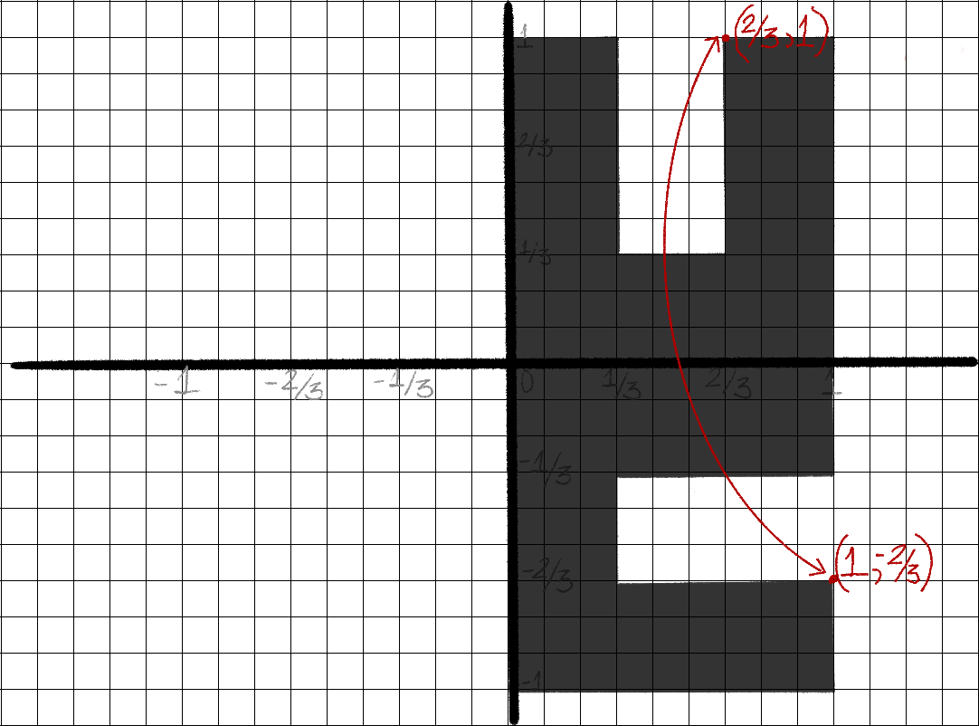
A light trigonometry intermission
y_new = -y_old & x_new = -x_old
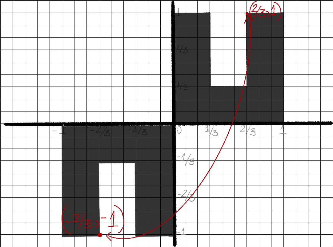
A light trigonometry intermission
y_new = x_old & x_new = -y_old
A light trigonometry intermission
- Step 1: Place shape
- Step 2: Subtract point of rotation off of each vertex
- Step 3: Rotate
- Step 4: Add back point of rotation
- Step 5: Correct coordinates to back at “original origin”
Applying trigonometry lesson
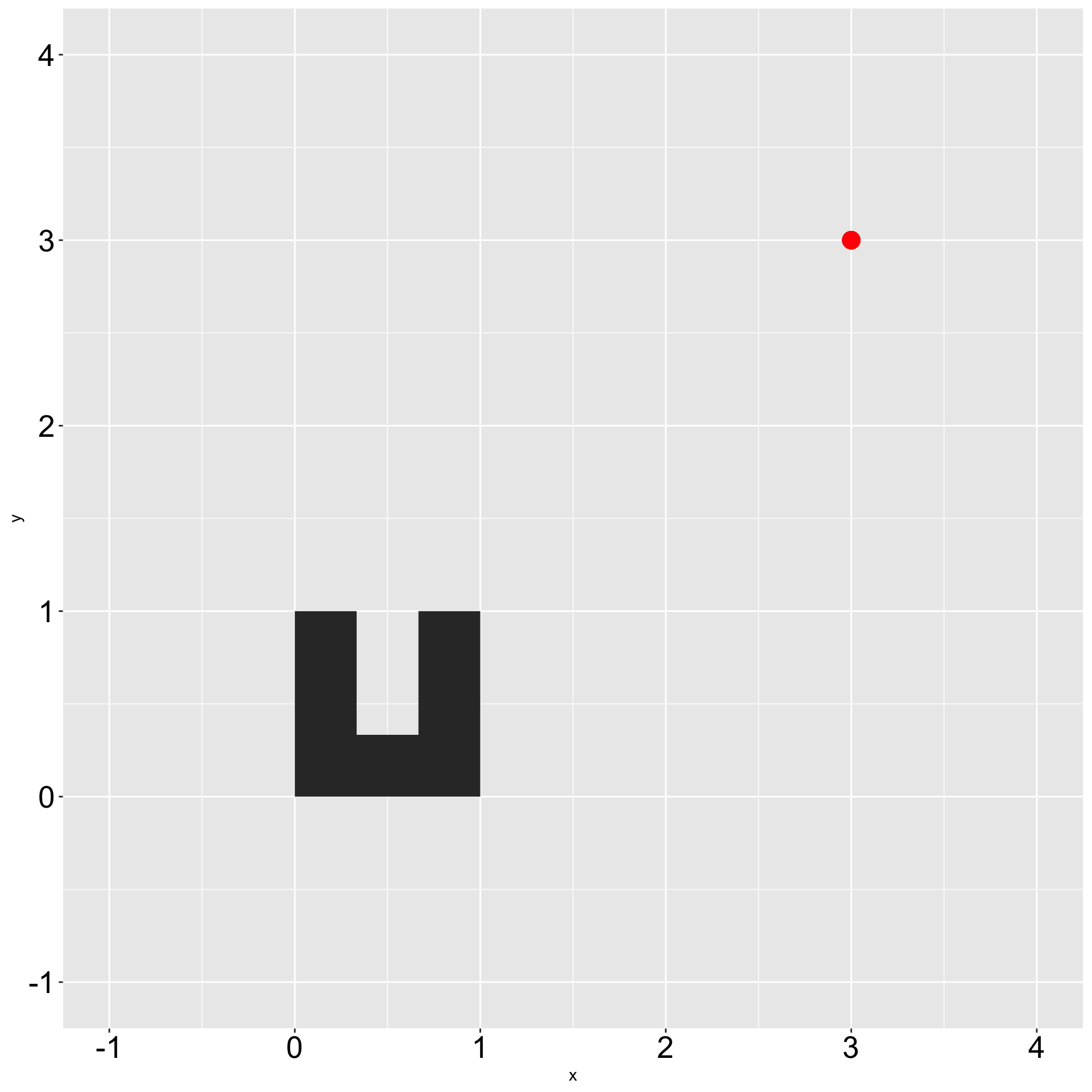
Step 1: Place shape
Applying trigonometry lesson
Step 2: Subtract point of rotation off of each vertex
Applying trigonometry lesson
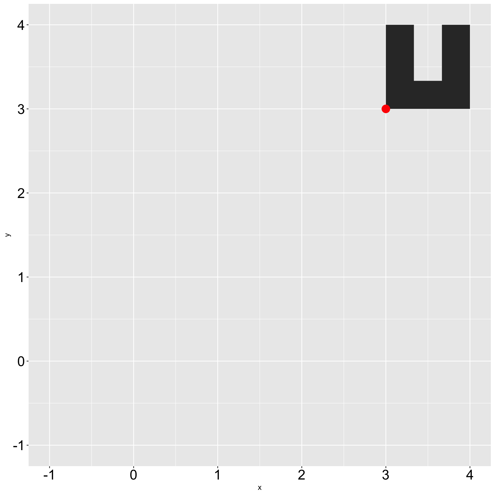
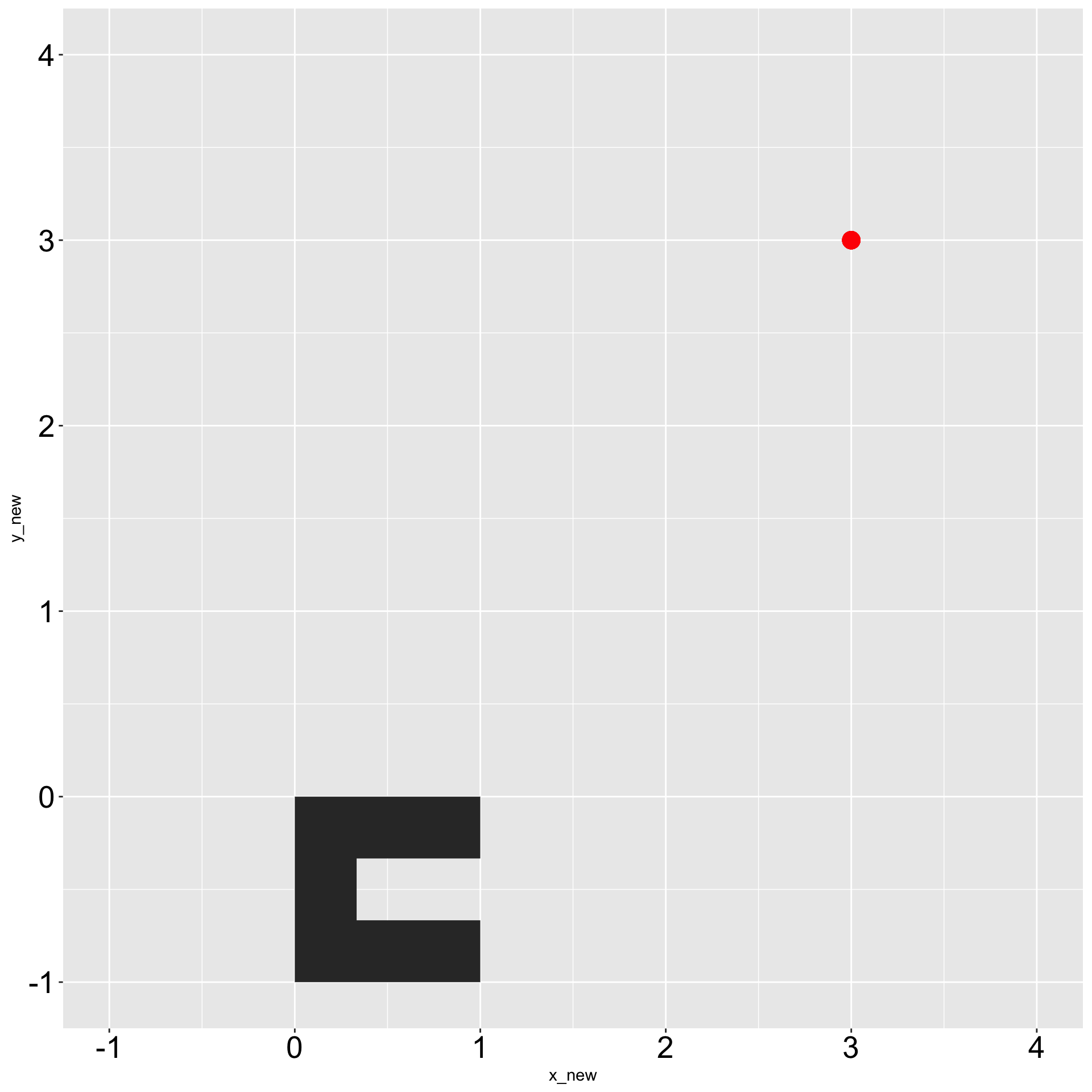
Step 3: Rotate
x0 <- 3
y0 <- 3

initial_u_shape <-
  create_initial_shape(x0, y0) %>%
  mutate(
    x = x - x0,
    y = y - y0
  ) %>%
  mutate(
    x_new = y,
    y_new = -x
  )

initial_u_shape %>%
  ggplot() +
  geom_polygon(
    aes(
      x = x_new,
      y = y_new
    )
  ) +
  geom_point(
    aes(
      x = x0,
      y = y0
    ),
    size = 5,
    color = "red"
  ) +
  coord_fixed(
    xlim = c(-1, 4),
    ylim = c(-1, 4)
  )
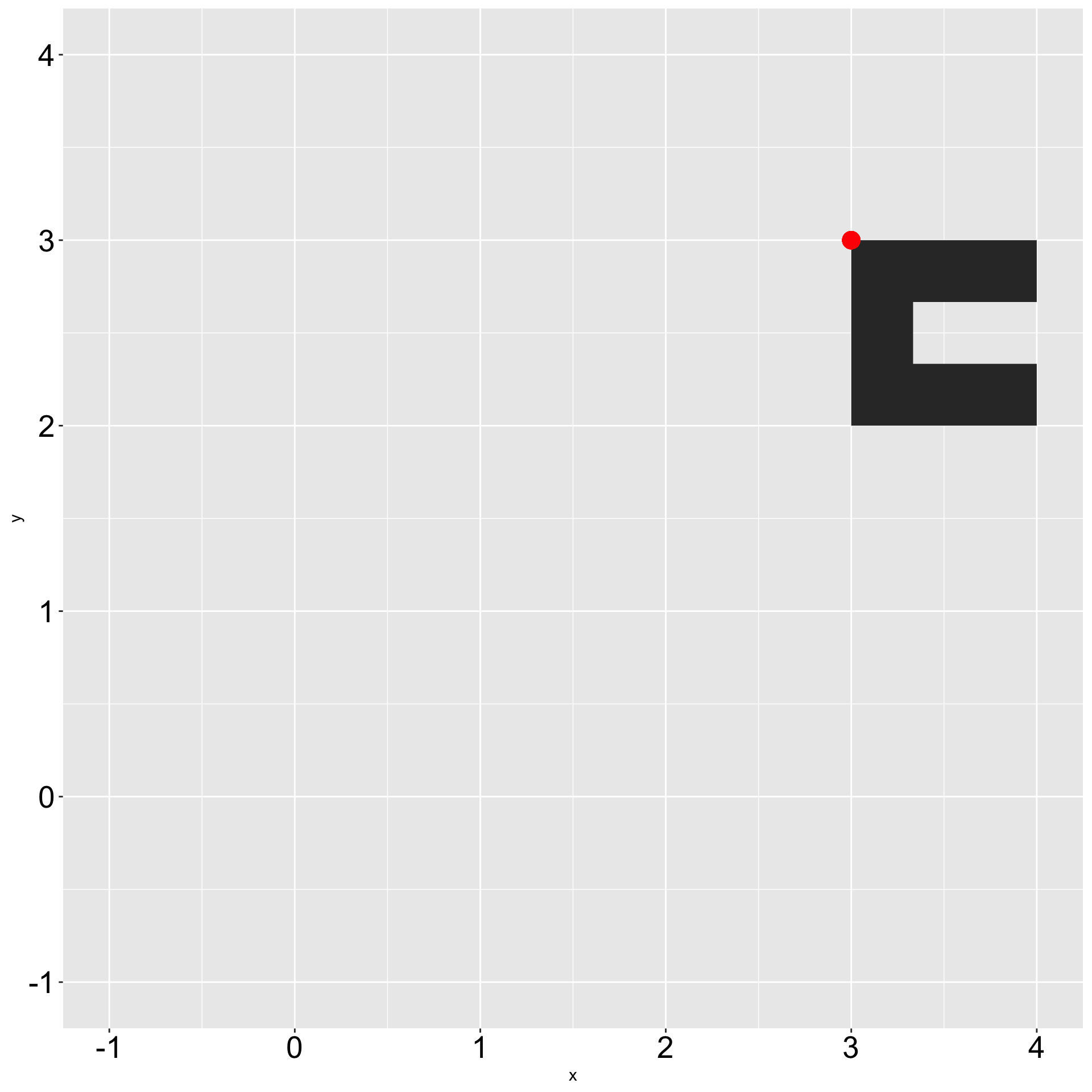
Applying trigonometry lesson
Step 4: Add back point of rotation
x0 <- 3
y0 <- 3

initial_u_shape <-
  create_initial_shape(x0, y0) %>%
  mutate(
    x = x - x0,
    y = y - y0
  ) %>%
  mutate(
    x_new = y,
    y_new = -x
  ) %>%
  mutate(
    x = x_new + x0,
    y = y_new + y0
  )

initial_u_shape %>%
  ggplot() +
  geom_polygon(
    aes(
      x = x,
      y = y
    )
  ) +
  geom_point(
    aes(
      x = x0,
      y = y0
    ),
    size = 5,
    color = "red"
  ) +
  coord_fixed(
    xlim = c(-1, 4),
    ylim = c(-1, 4)
  )
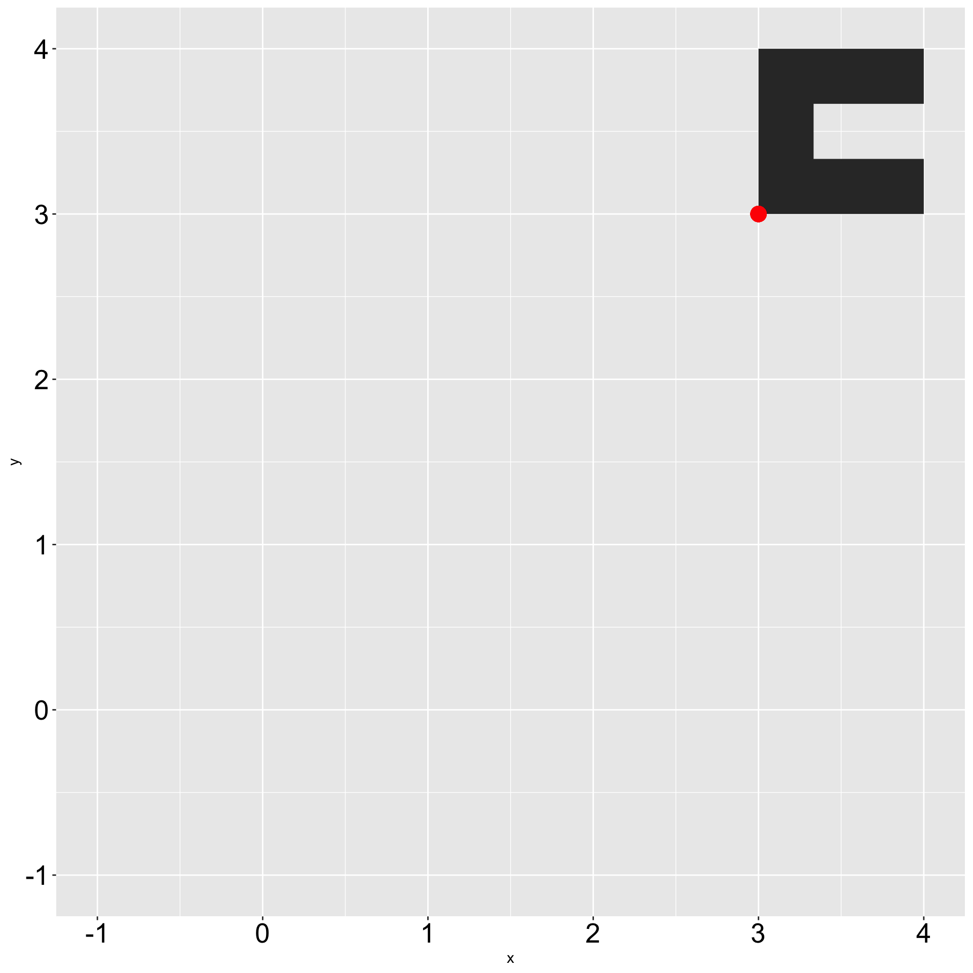
Applying trigonometry lesson
Step 5: Correct coordinates to back at “original origin”
x0 <- 3
y0 <- 3
shape_width <- 1

initial_u_shape <-
  create_initial_shape(x0, y0) %>%
  mutate(
    x = x - x0,
    y = y - y0
  ) %>%
  mutate(
    x_new = y,
    y_new = -x
  ) %>%
  mutate(
    x = x_new + x0,
    y = y_new + y0 + shape_width
  )

initial_u_shape %>%
  ggplot() +
  geom_polygon(
    aes(
      x = x,
      y = y
    )
  ) +
  geom_point(
    aes(
      x = x0,
      y = y0
    ),
    size = 5,
    color = "red"
  ) +
  coord_fixed(
    xlim = c(-1, 4),
    ylim = c(-1, 4)
  )
Turning lesson[s] into function[s]
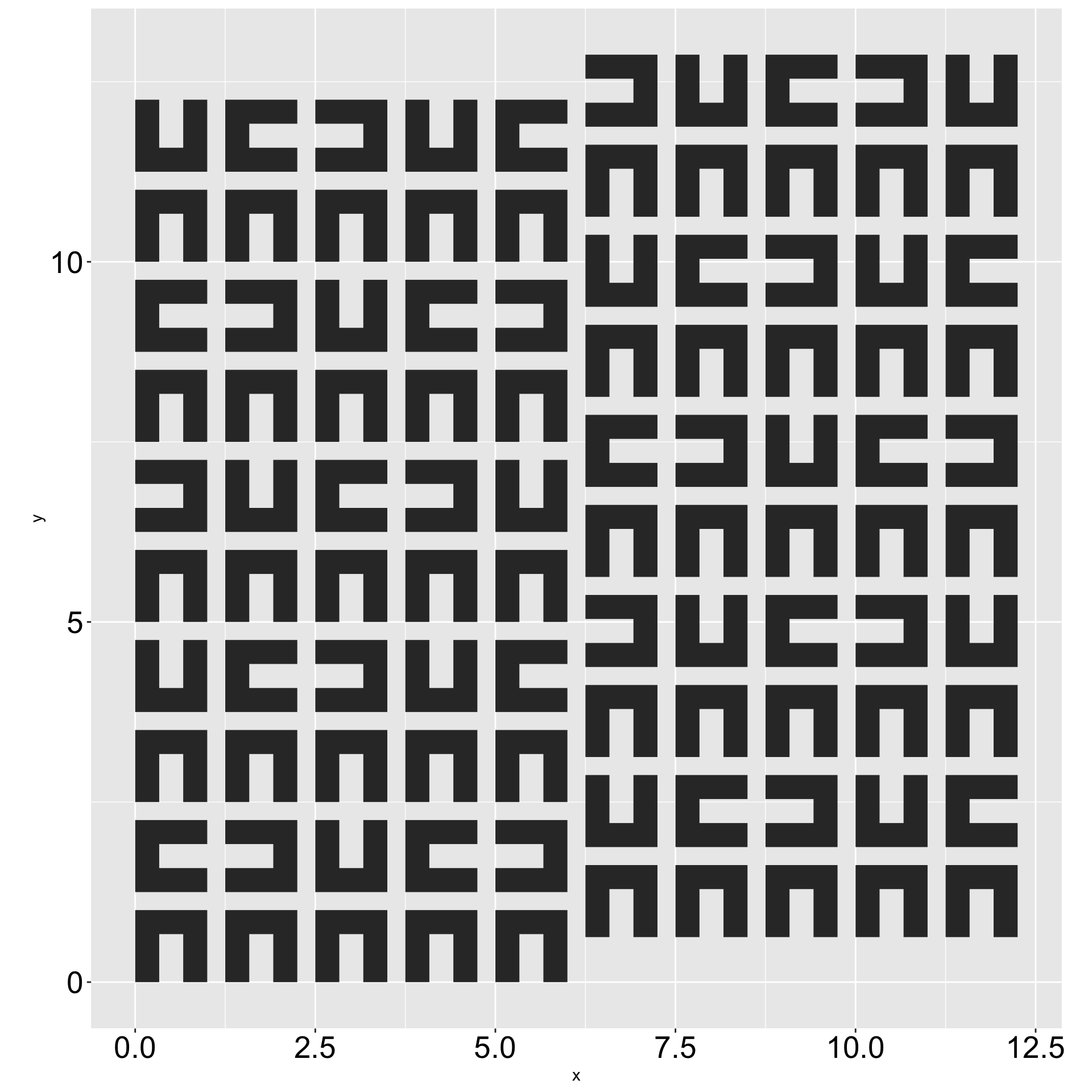
Creating the grid
Creating the grid
ncol <- 10
nrow <- 10
shape_width <- 1
perimeter_width <- shape_width + .25
grid <-
expand_grid(
x = seq(0,
by = perimeter_width,
length.out = ncol
),
y = seq(0,
by = perimeter_width,
length.out = nrow
)
) %>%
mutate(y = if_else(x >= 5 * perimeter_width,
y + perimeter_width / 2,
y
))
grid# A tibble: 100 × 2
x y
<dbl> <dbl>
1 0 0
2 0 1.25
3 0 2.5
4 0 3.75
5 0 5
6 0 6.25
7 0 7.5
8 0 8.75
9 0 10
10 0 11.2
# ℹ 90 more rows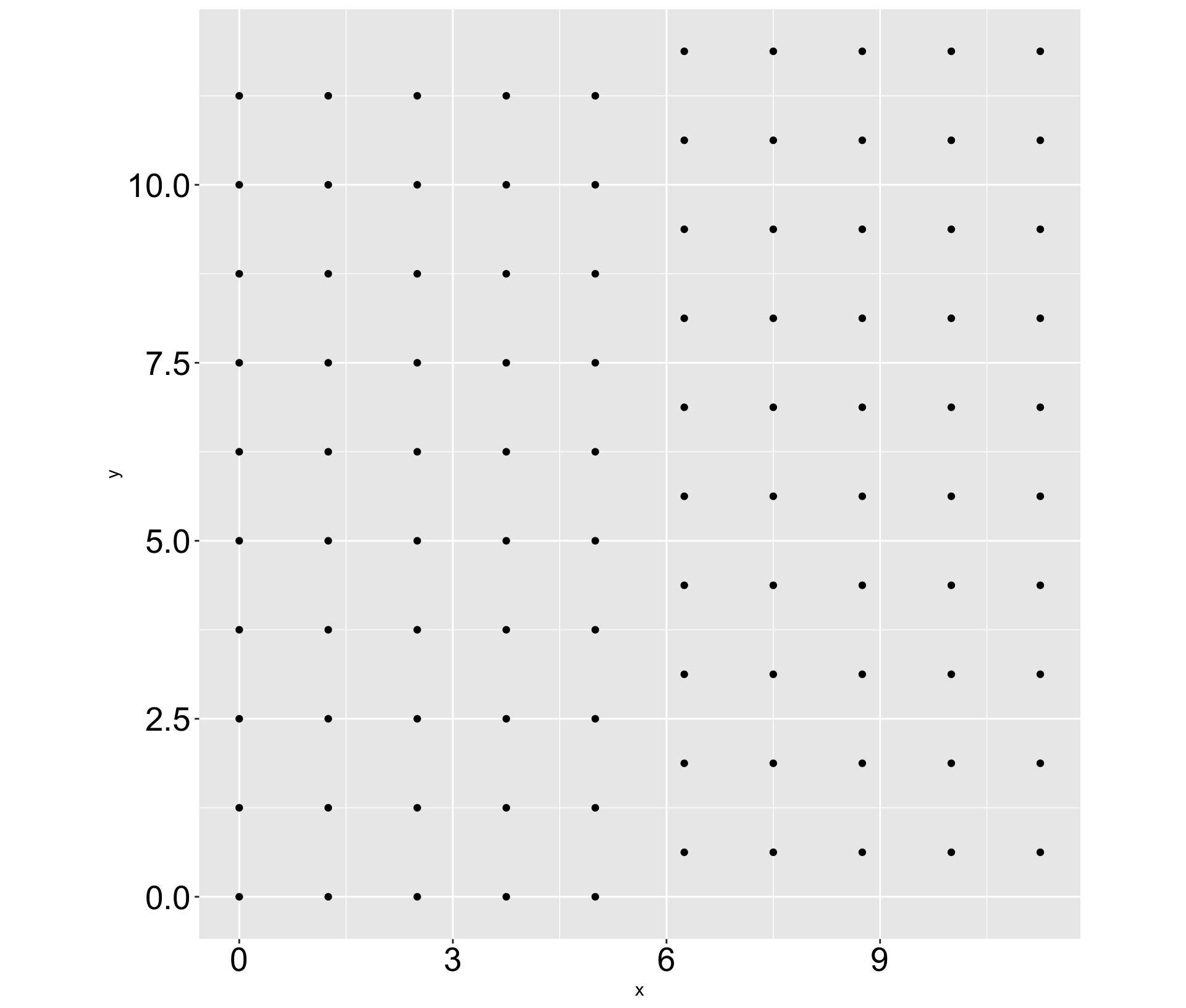
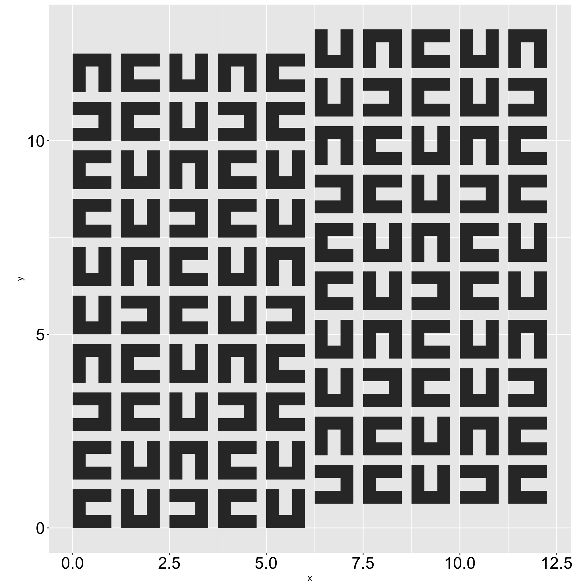
Applying our system
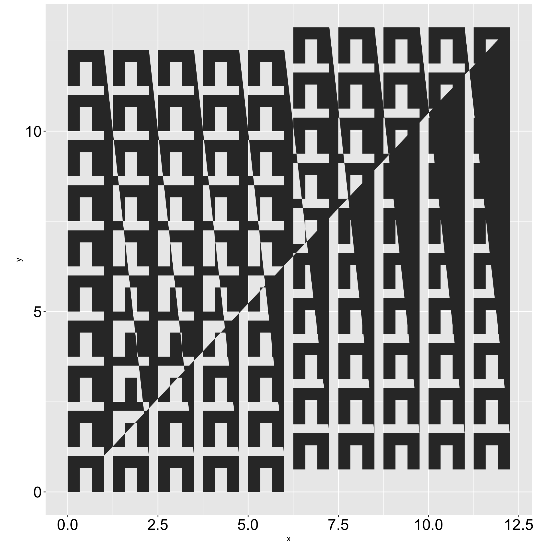
Applying our system
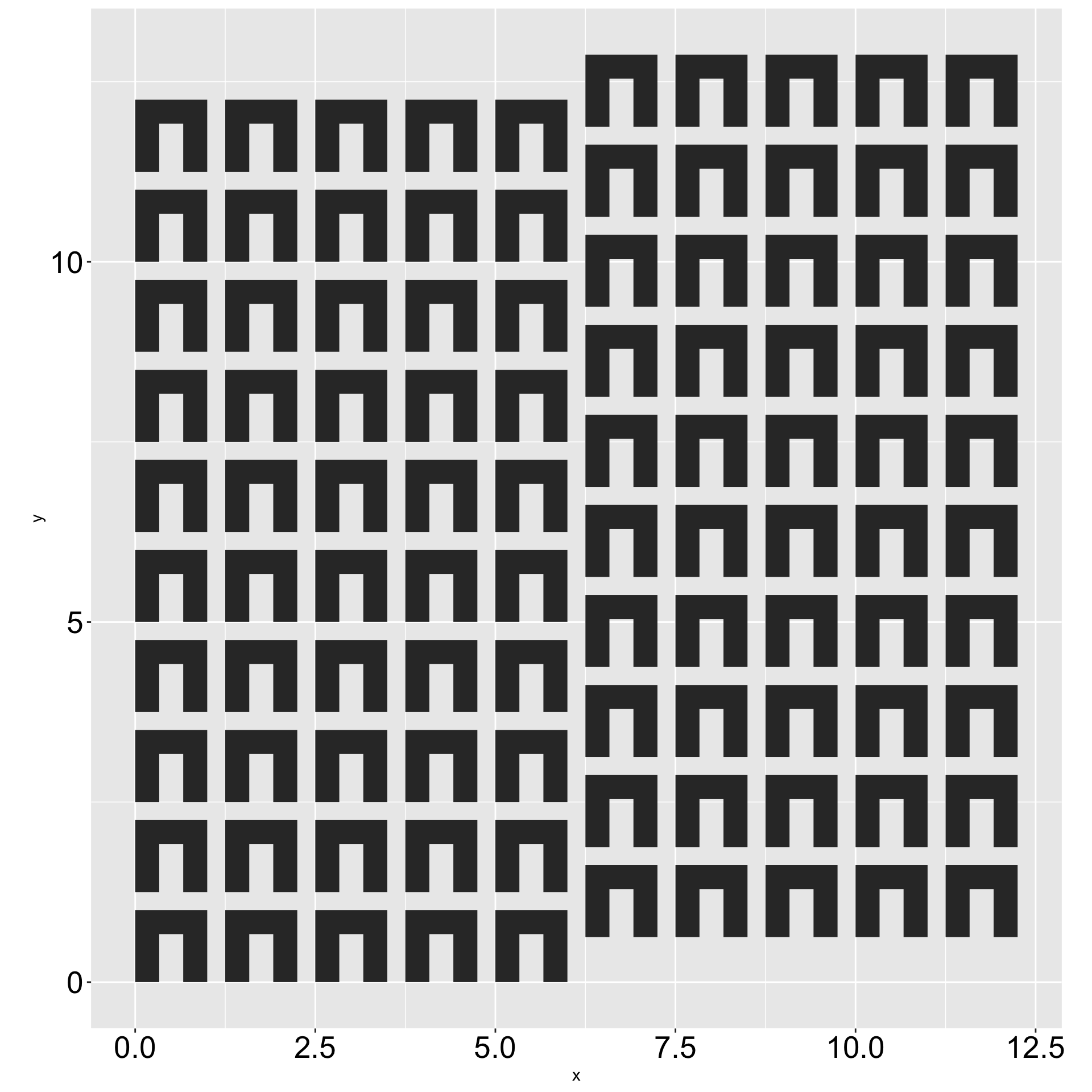
Applying our system
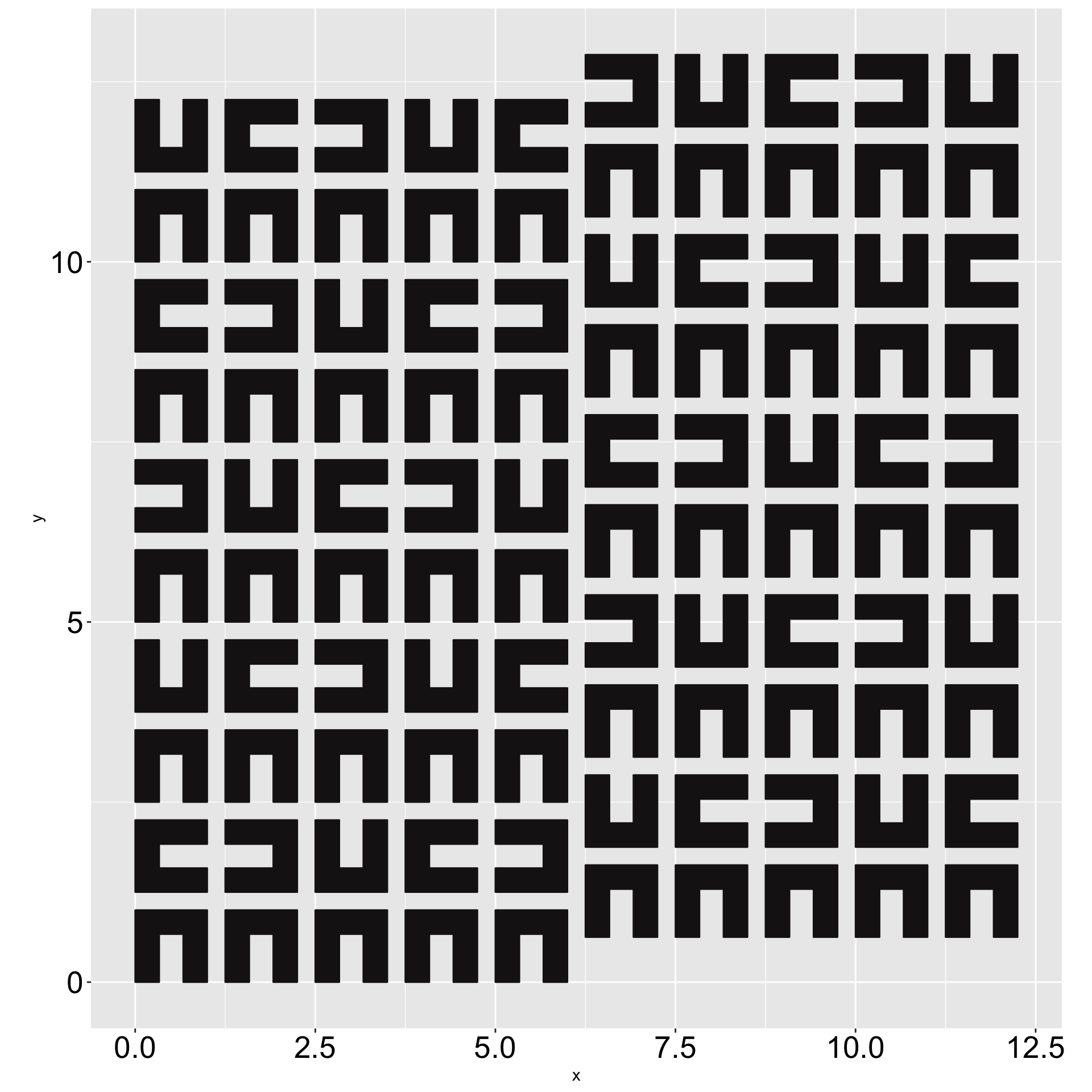
Incorporating rotation
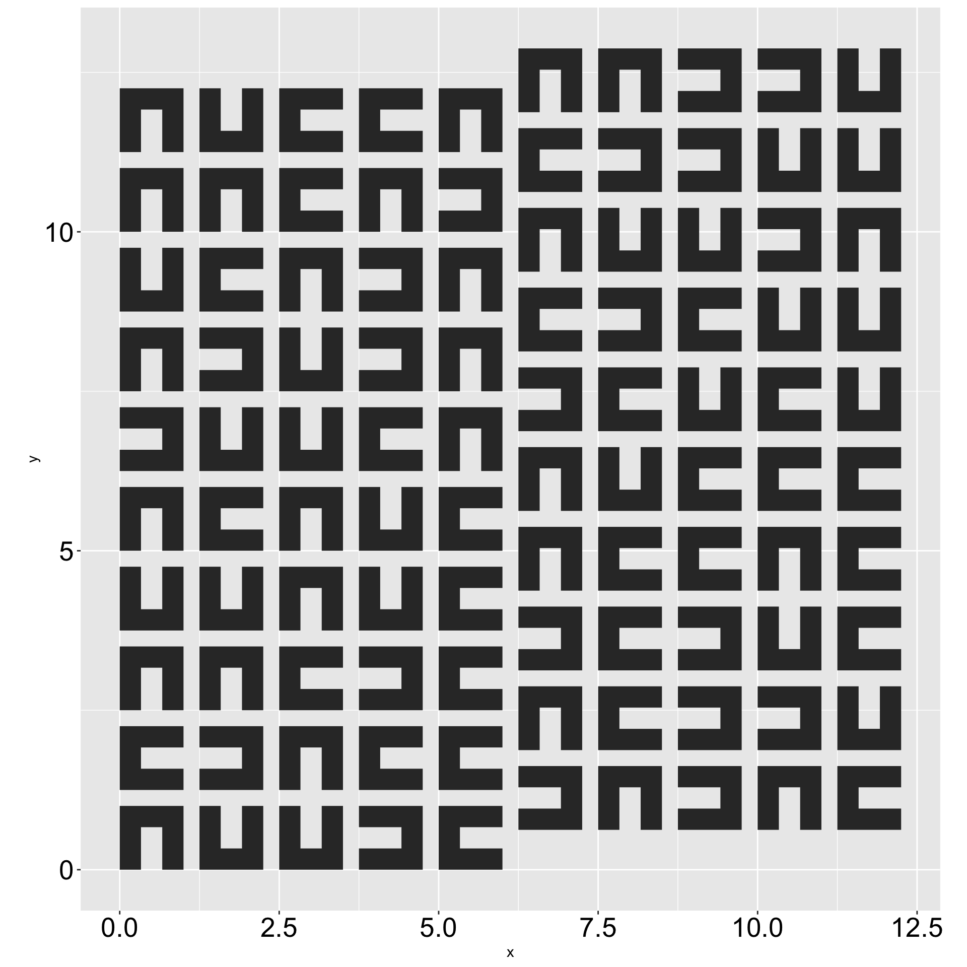
Patterns vs. Pure Random
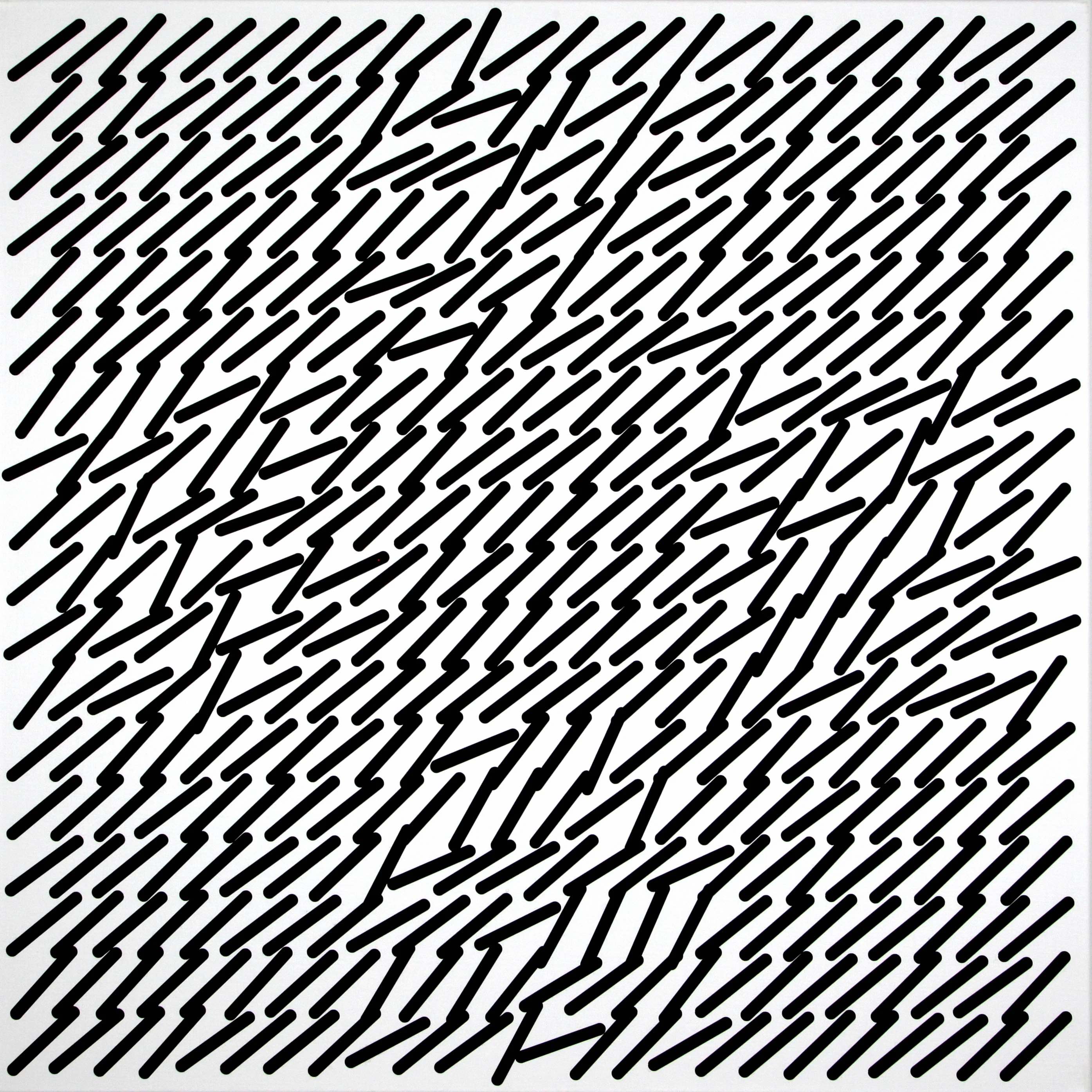
Patterns vs. Pure Random


Patterns vs. Pure Random
Layout: 1, 2, 3, Skip, 4, 1, 2
Patterns vs. Pure Random
Patterns vs. Pure Random
Final Piece
Final Piece
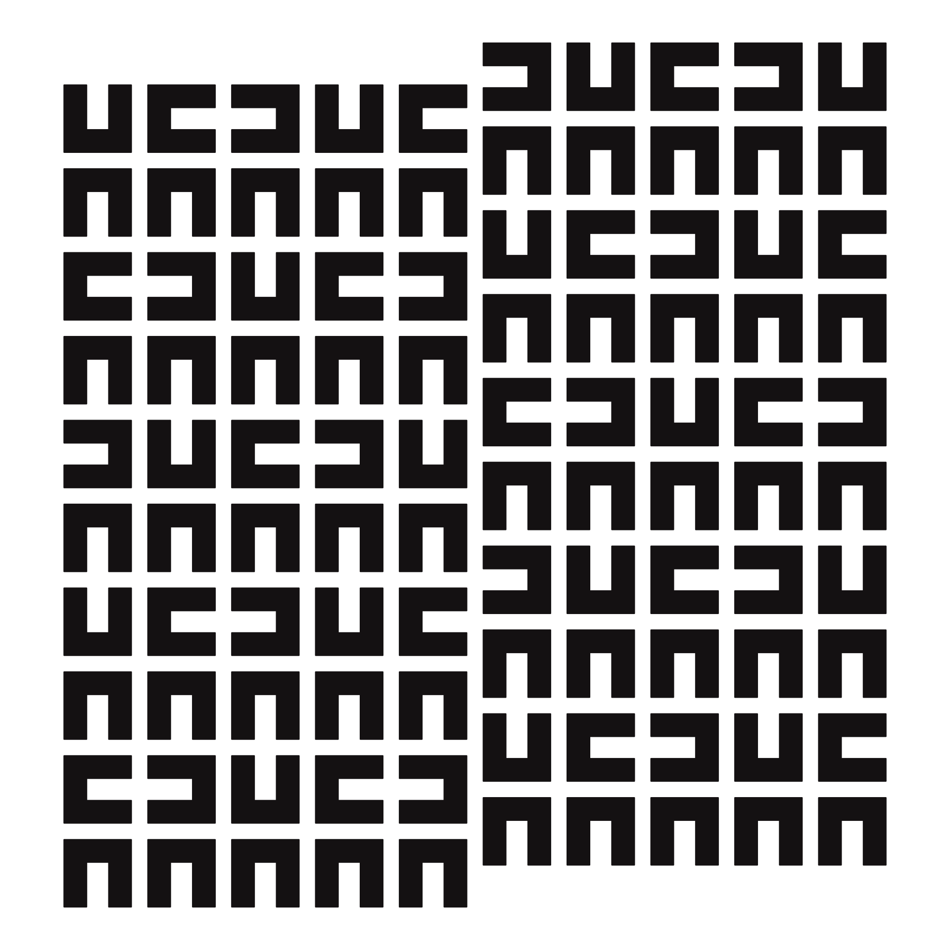
Final Piece

Final Piece