library(ggplot2)
library(dplyr)
library(stringr)

bikes <- readr::read_csv(
  here::here("data", "london-bikes-custom.csv"),
  col_types = "Dcfffilllddddc"
)

theme_set(theme_light(base_size = 14, base_family = "Asap SemiCondensed"))

theme_update(
  panel.grid.minor = element_blank(),
  plot.title = element_text(face = "bold"),
  plot.title.position = "plot"
)Engaging and Beautiful Data Visualizations with ggplot2
Working with Text
Working with Labels
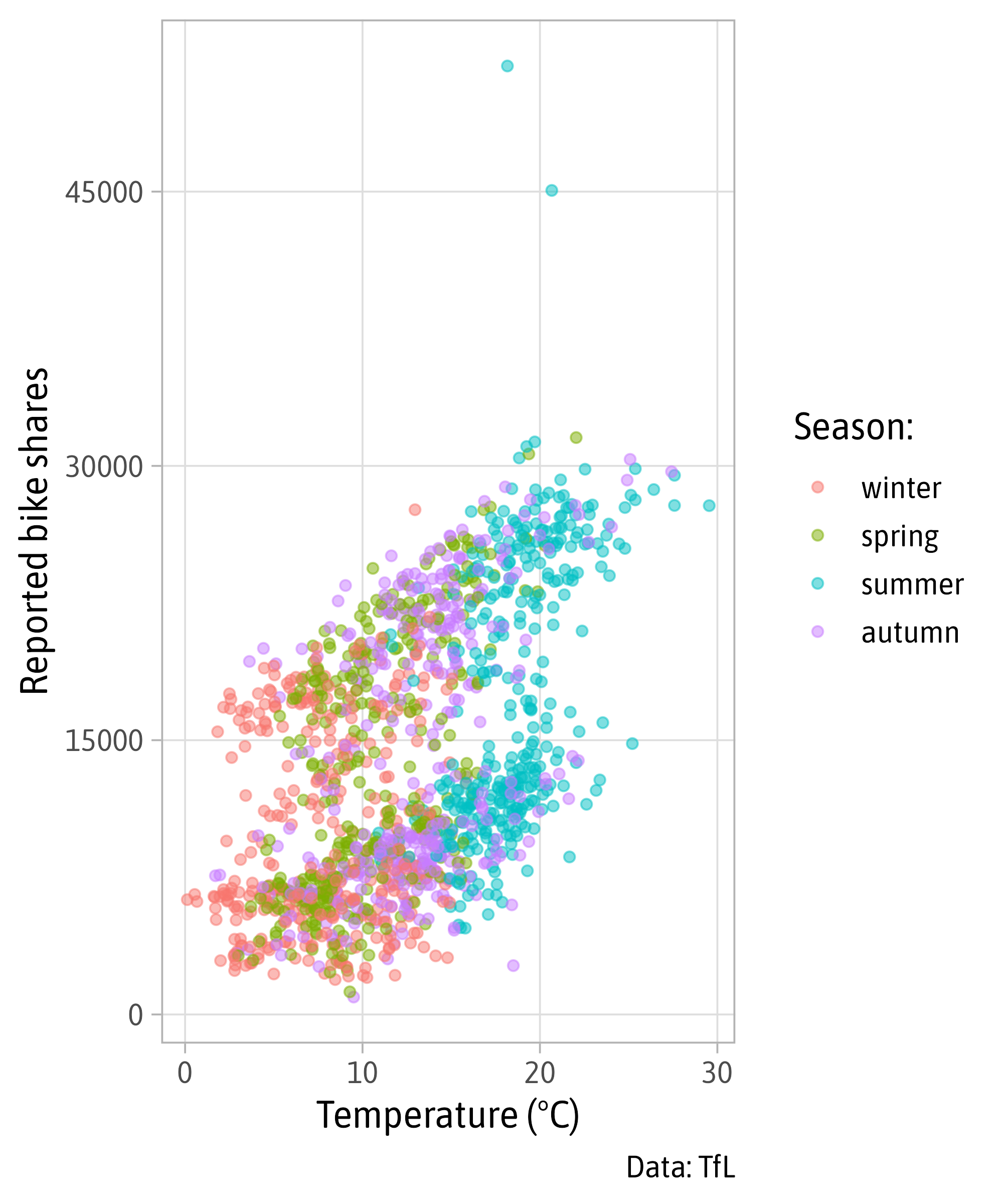
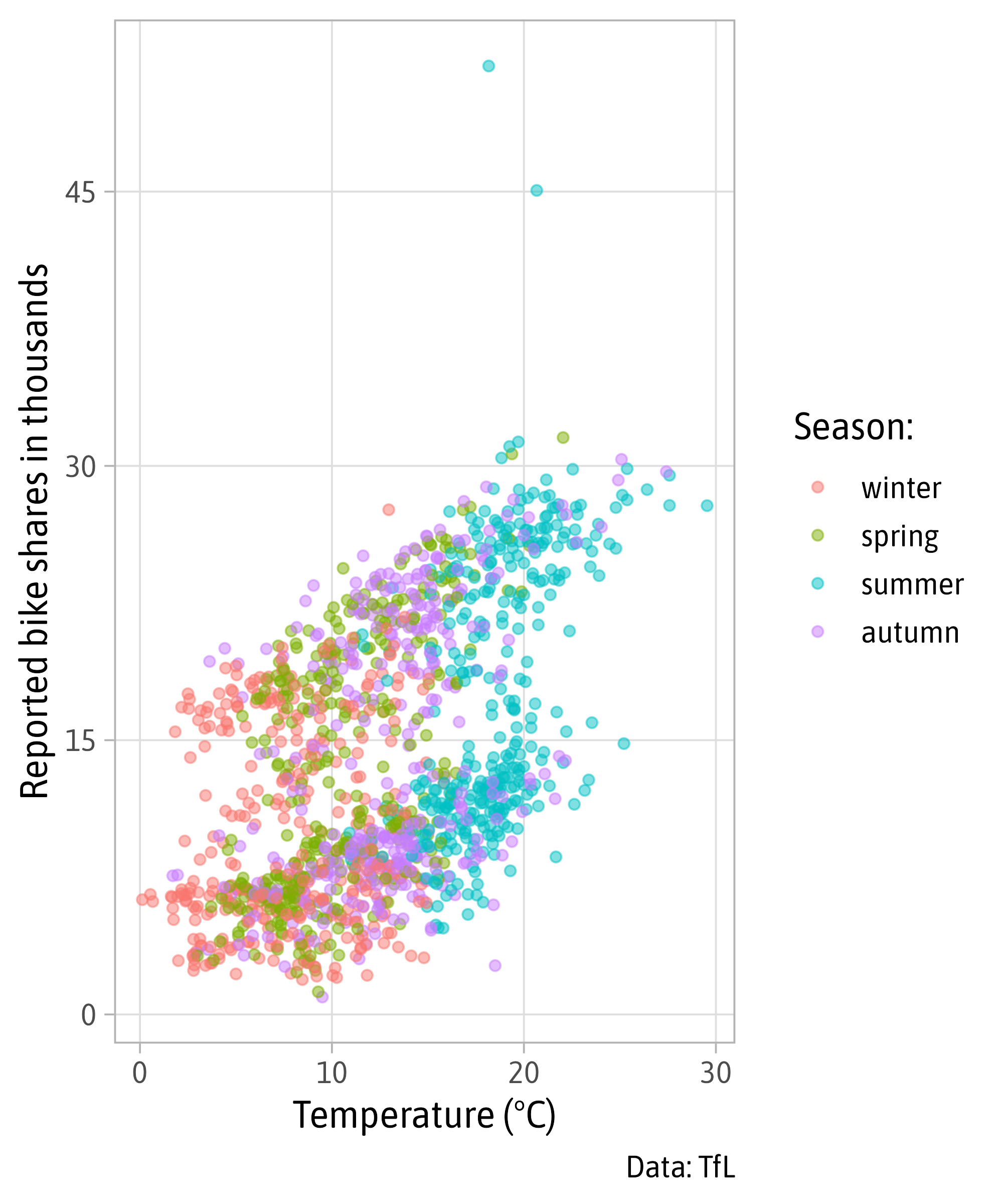
g <- ggplot(
    bikes,
    aes(x = temp, y = count,
        color = season)
  ) +
  geom_point(
    alpha = .5
  ) +
  labs(
    x = "Temperature (°C)",
    y = "Reported bike shares",
    title = "TfL bike sharing trends",
    subtitle = "Reported bike rents versus air temperature in London",
    caption = "Data: TfL",
    color = "Season:",
    tag = "1."
  )

g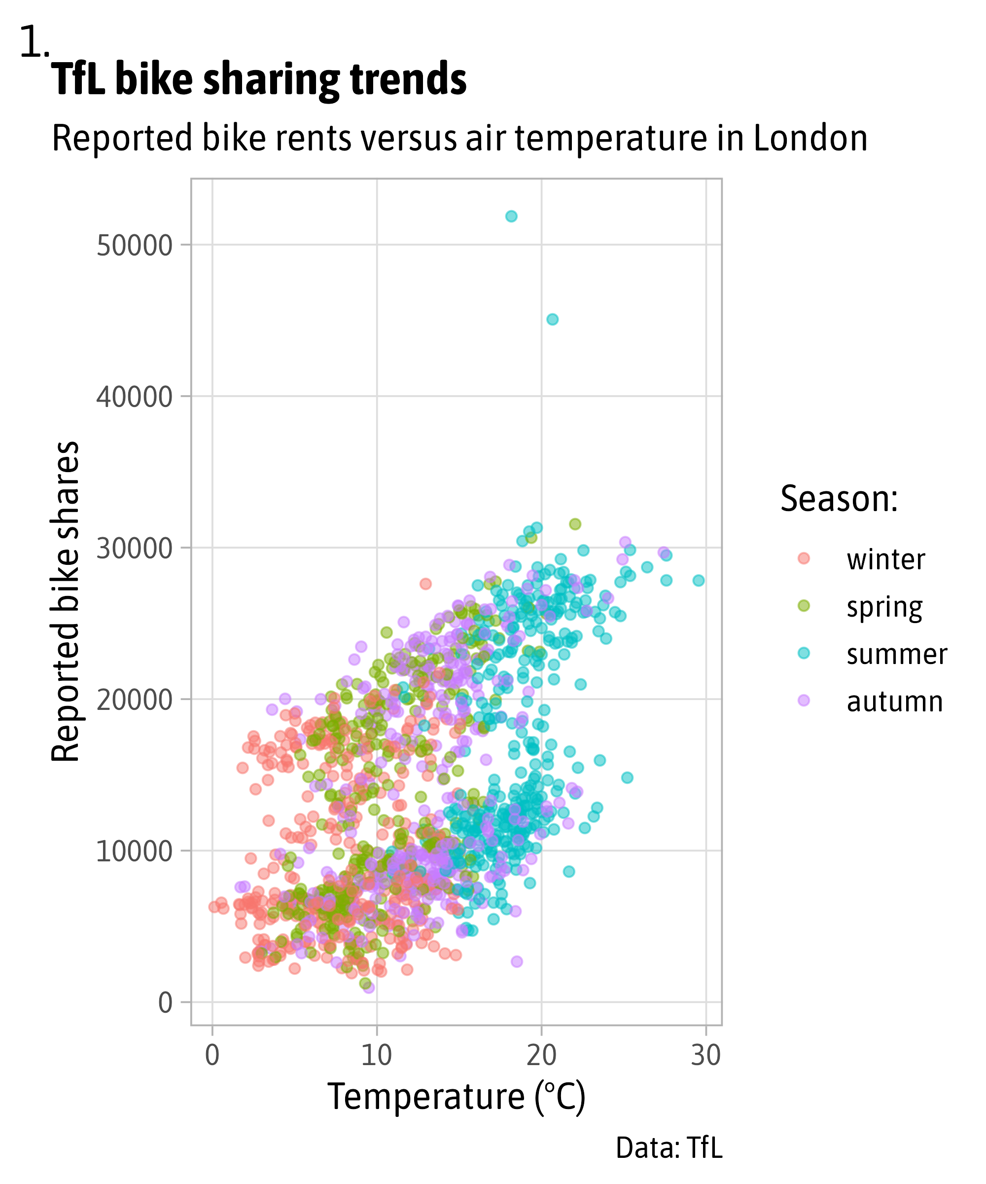
Customize Labels via theme()

Customize Labels via theme()

Customize Labels via theme()

Customize Labels via theme()
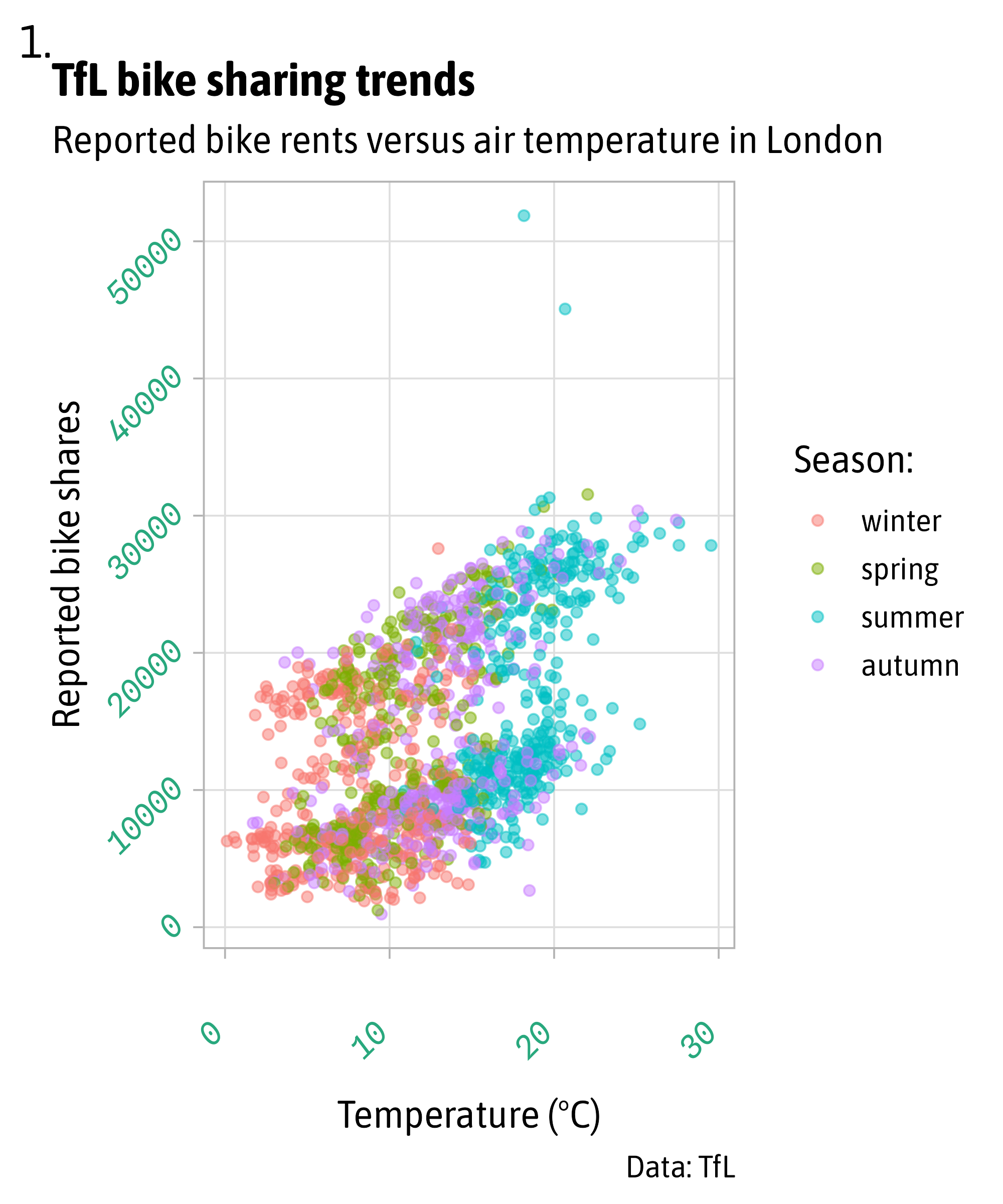
g + theme(
  plot.title = element_text(face = "bold"),
  plot.title.position = "plot",
  axis.text = element_text(
    color = "#28a87d",
    family = "Spline Sans Mono",
    face = "italic",
    lineheight = 1.3, # no effect here
    angle = 45,
    hjust = 1, # no effect here
    vjust = 0, # no effect here
    margin = margin(10, 0, 20, 0) # no effect here
  )
)
Customize Labels via theme()
g + theme(
plot.title = element_text(face = "bold"),
plot.title.position = "plot",
axis.text = element_text(
color = "#28a87d",
family = "Spline Sans Mono",
face = "italic",
lineheight = 1.3, # no effect here
angle = 45,
hjust = 1, # no effect here
vjust = 0, # no effect here
margin = margin(10, 0, 20, 0) # no effect here
),
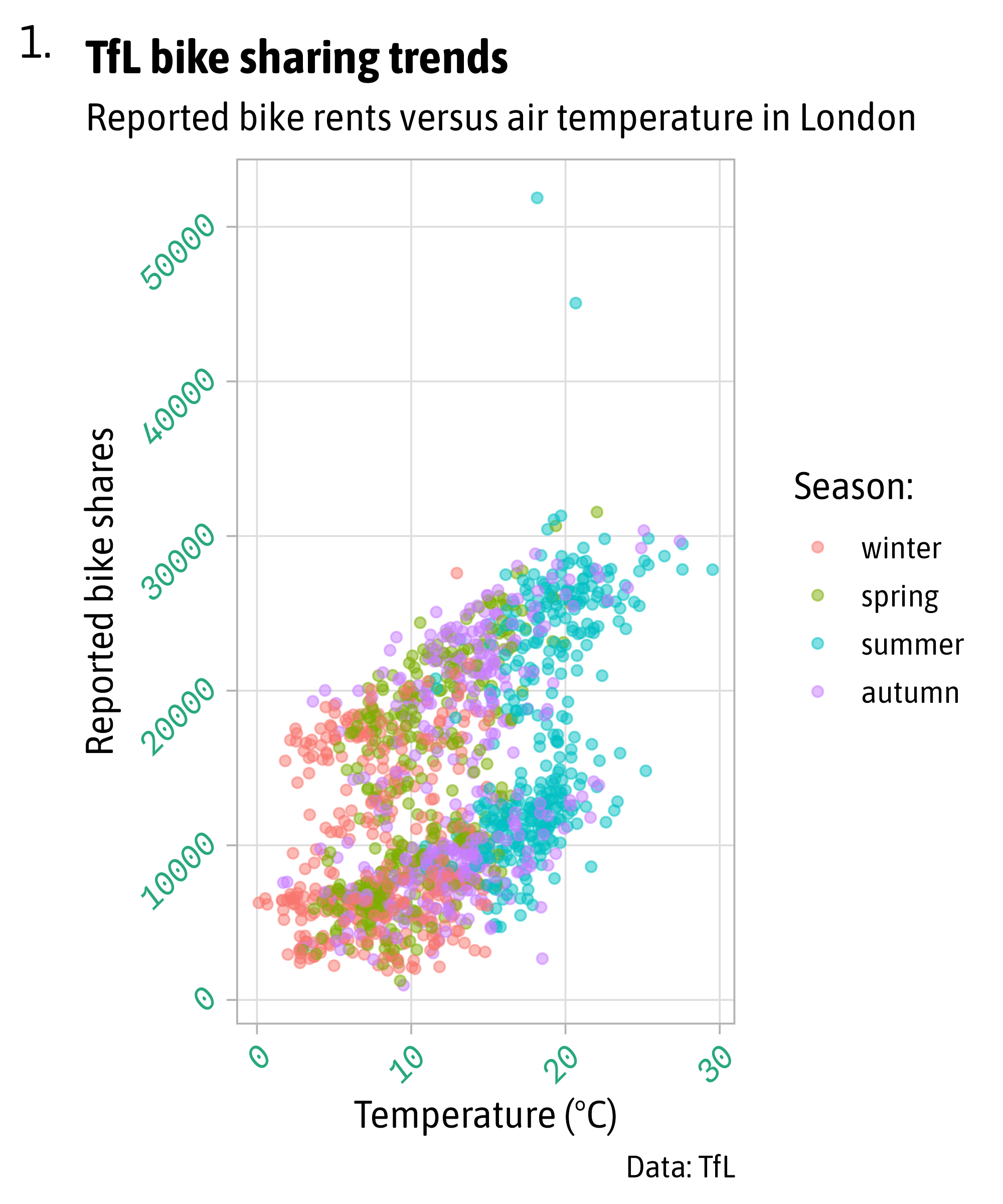
axis.text.x = element_text(
hjust = 1,
vjust = 0,
margin = margin(10, 0, 20, 0) # trbl
)
)
Customize Labels via theme()
g + theme(
  plot.title = element_text(face = "bold"),
  plot.title.position = "plot",
  axis.text = element_text(
    color = "#28a87d",
    family = "Spline Sans Mono",
    face = "italic",
    lineheight = 1.3, # no effect here
    angle = 45,
    hjust = 1, # no effect here
    vjust = 0, # no effect here
    margin = margin(10, 0, 20, 0) # no effect here
  ),
  plot.tag = element_text(
    margin = margin(0, 12, -8, 0) # trbl
  )
)
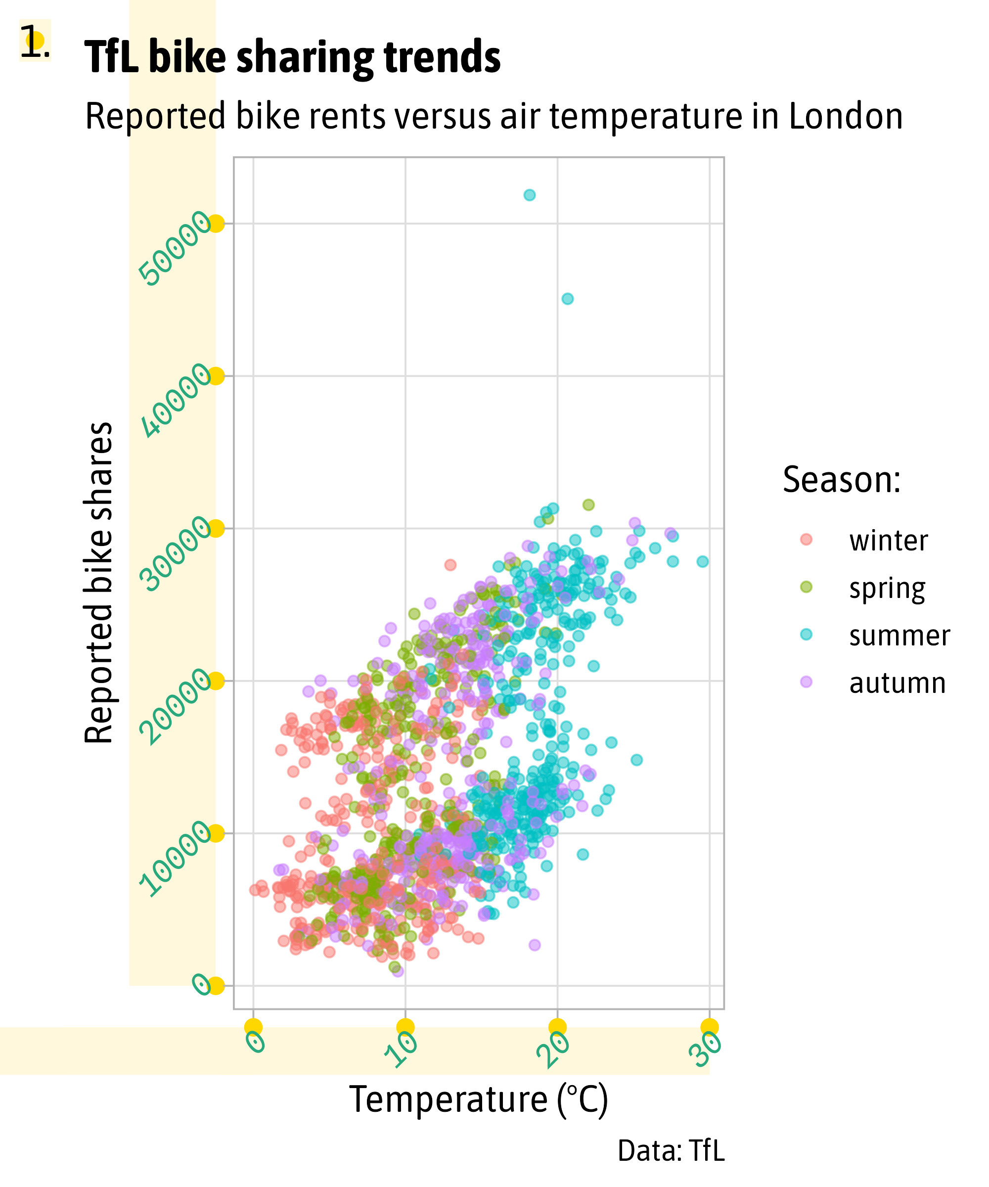
Customize Labels via theme()
g + theme(
  plot.title = element_text(face = "bold"),
  plot.title.position = "plot",
  axis.text = element_text(
    color = "#28a87d",
    family = "Spline Sans Mono",
    face = "italic",
    hjust = 1,
    vjust = 0,
    angle = 45,
    lineheight = 1.3, # no effect here
    margin = margin(10, 0, 20, 0), # no effect here
    debug = TRUE
  ),
  plot.tag = element_text(
    margin = margin(0, 12, -8, 0), # trbl
    debug = TRUE
  )
)
Format Labels via scale_*
Format Labels via scale_*
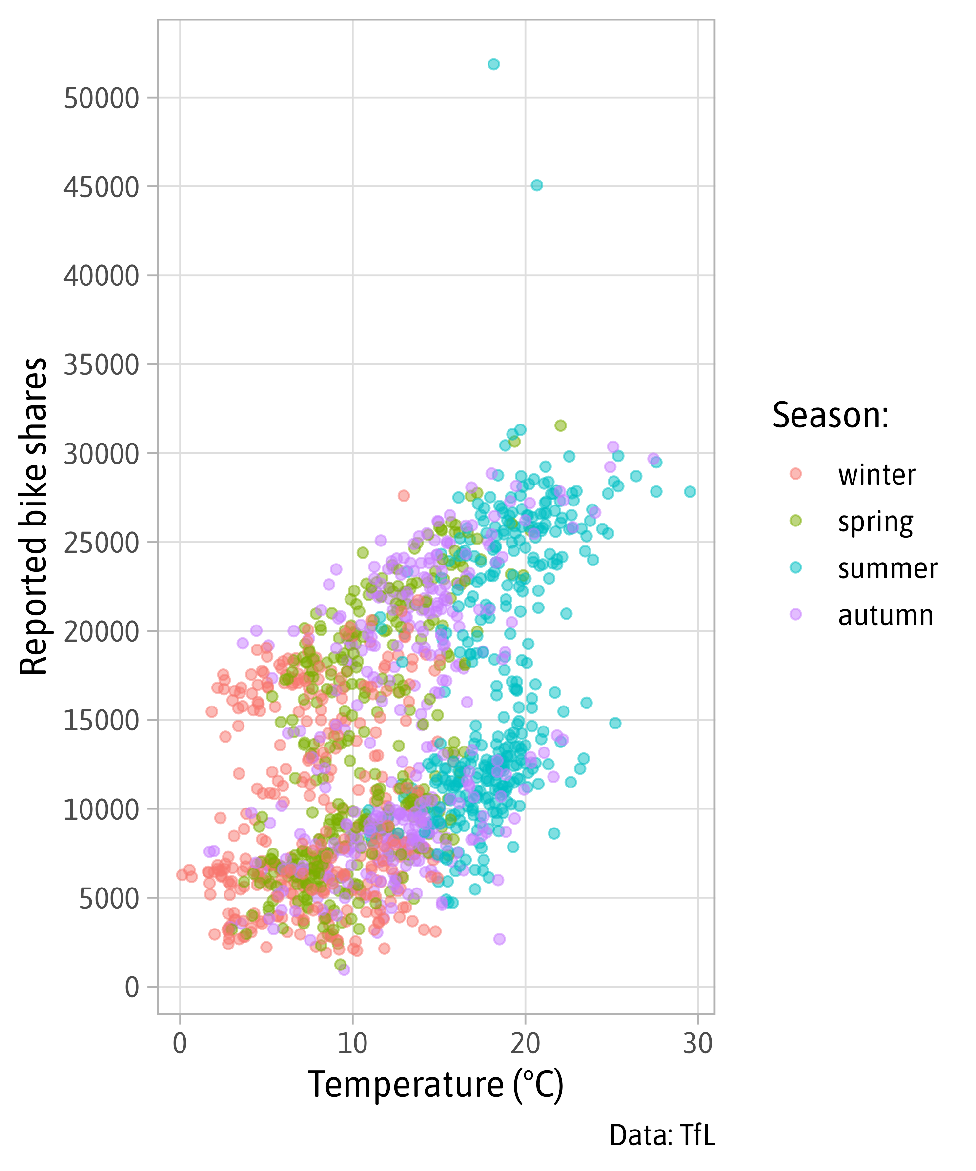
Format Labels via scale_*
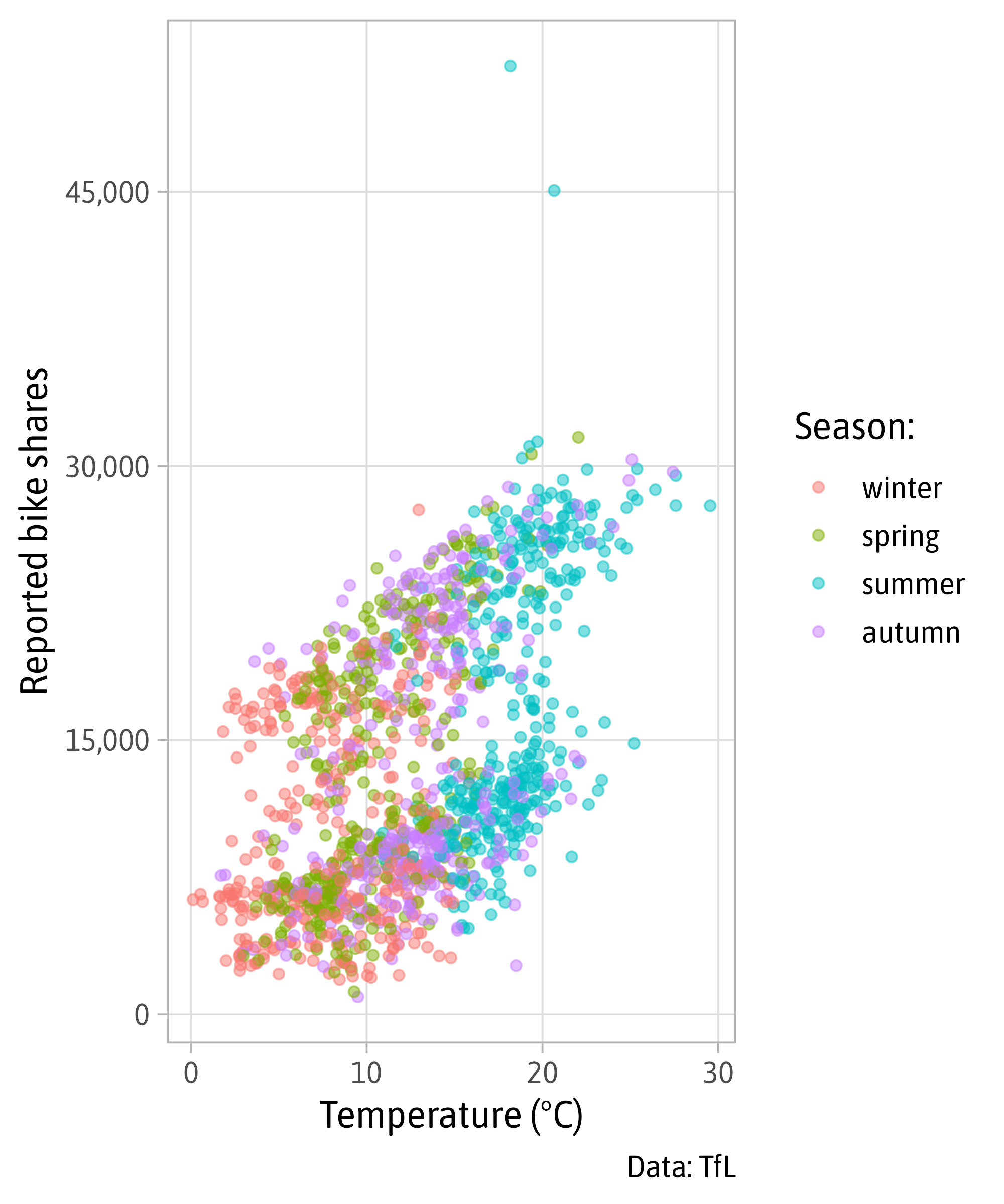
Format Labels via scale_*
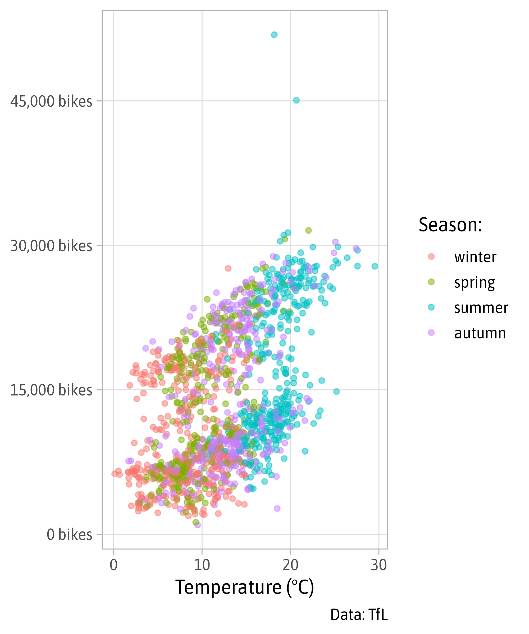
Format Labels via scale_*

Format Labels via scale_*
Format Labels via scale_*
Format Labels via scale_*

Styling Labels with {ggtext}
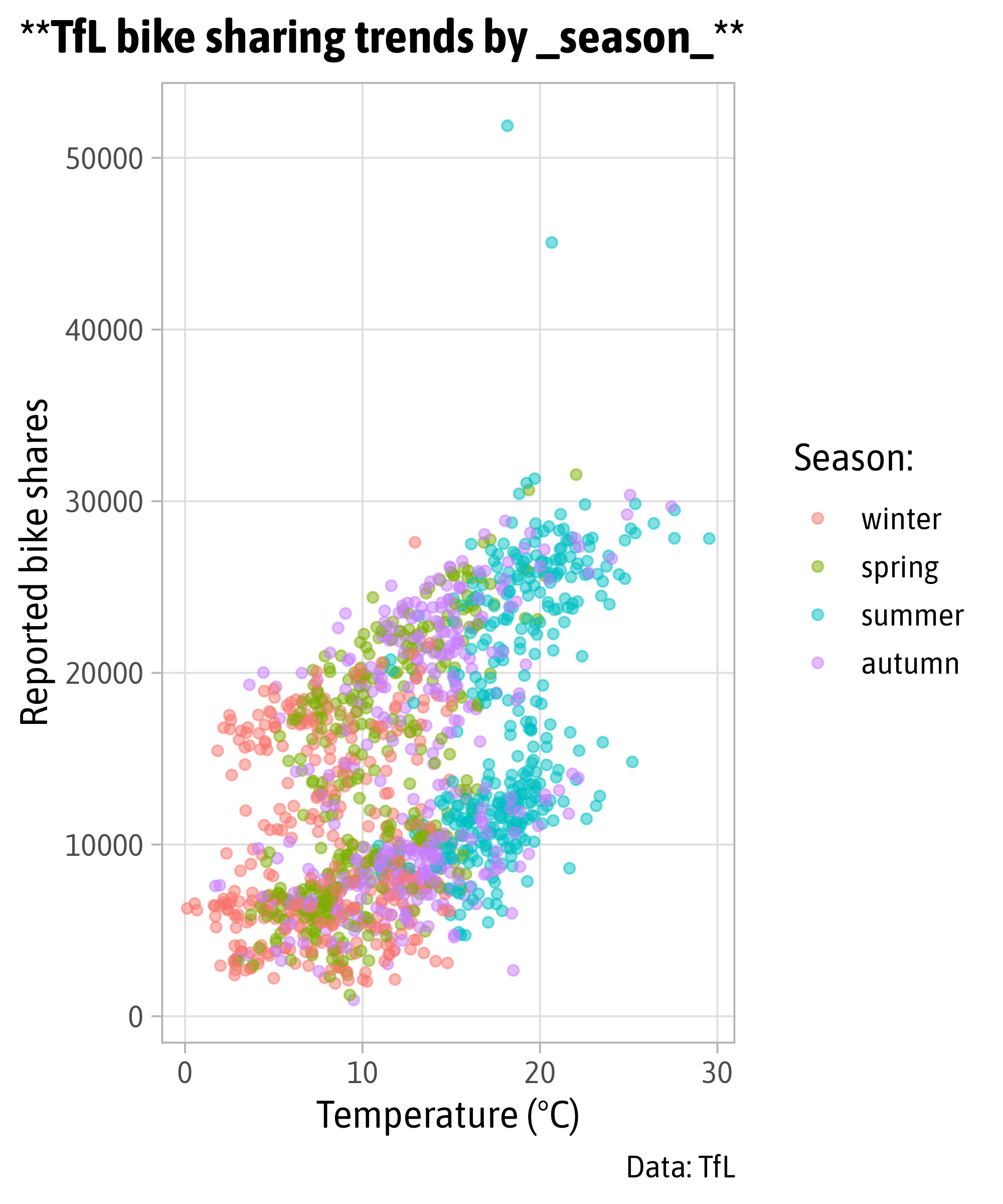
Styling Labels with {ggtext}
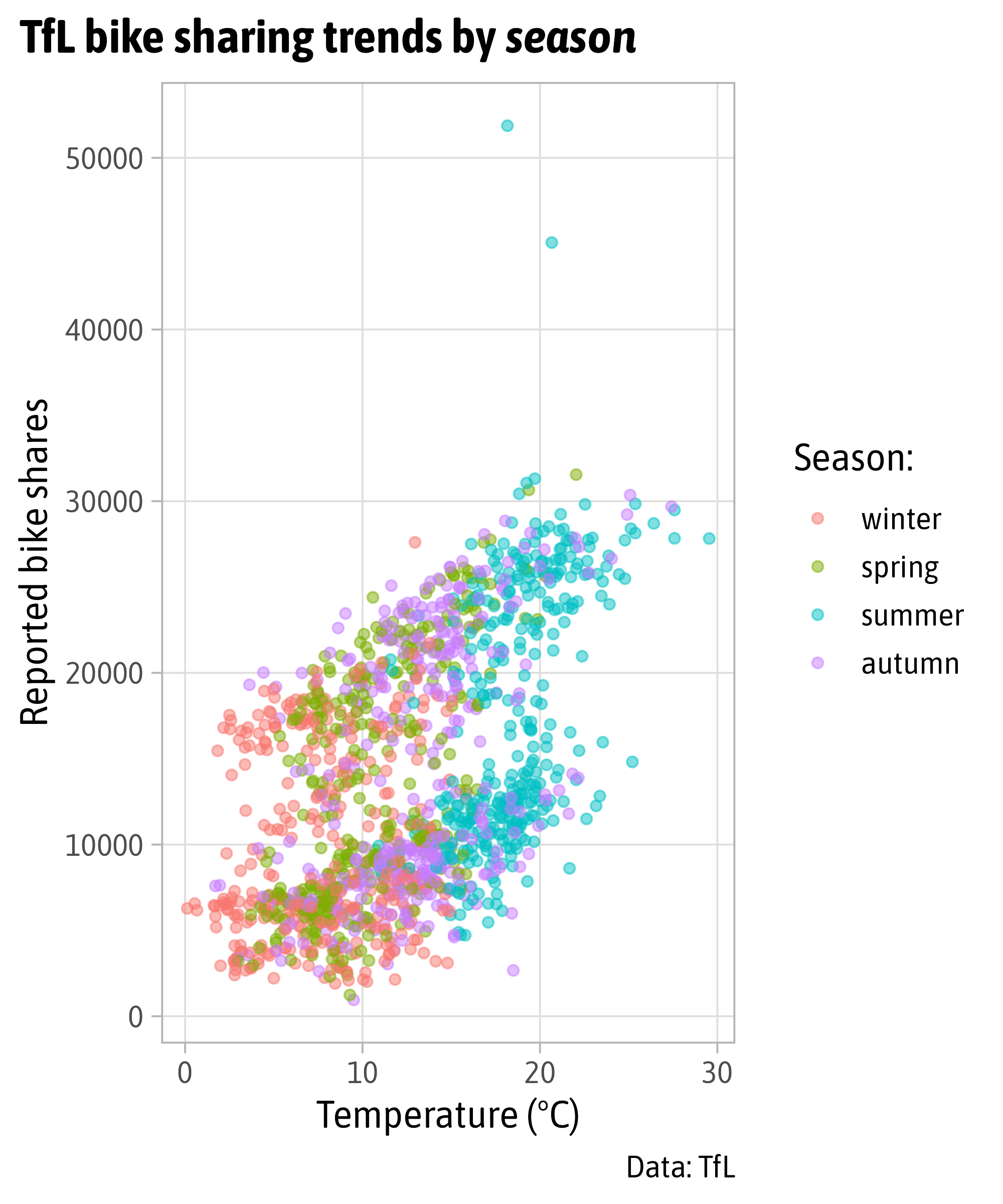
Styling Labels with {ggtext}

<b style='font-family:Times;font-size:25pt;'>TfL</b> bike sharing trends by <i style='color:#28A87;'>season</i>
Styling Labels with {ggtext}
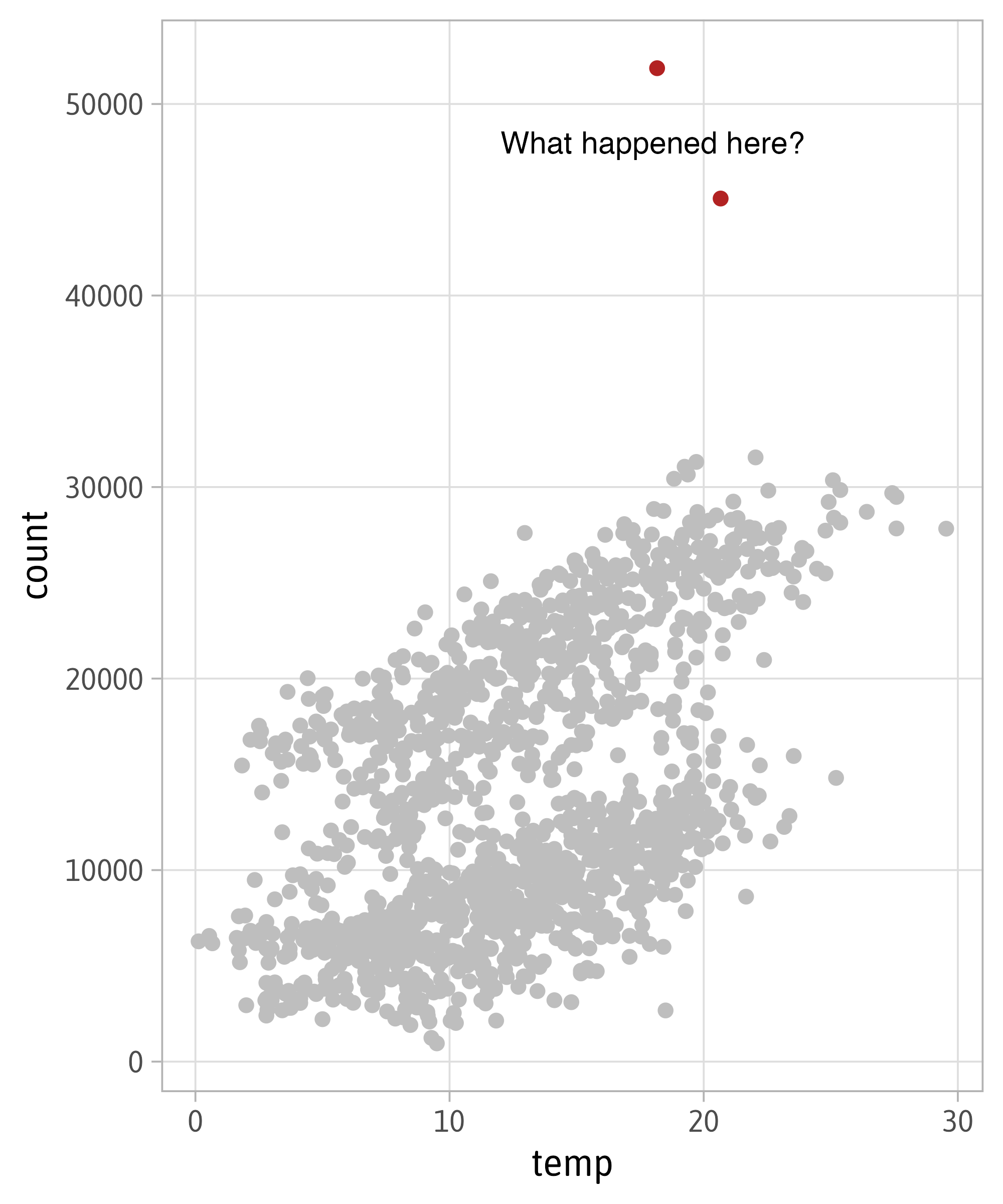
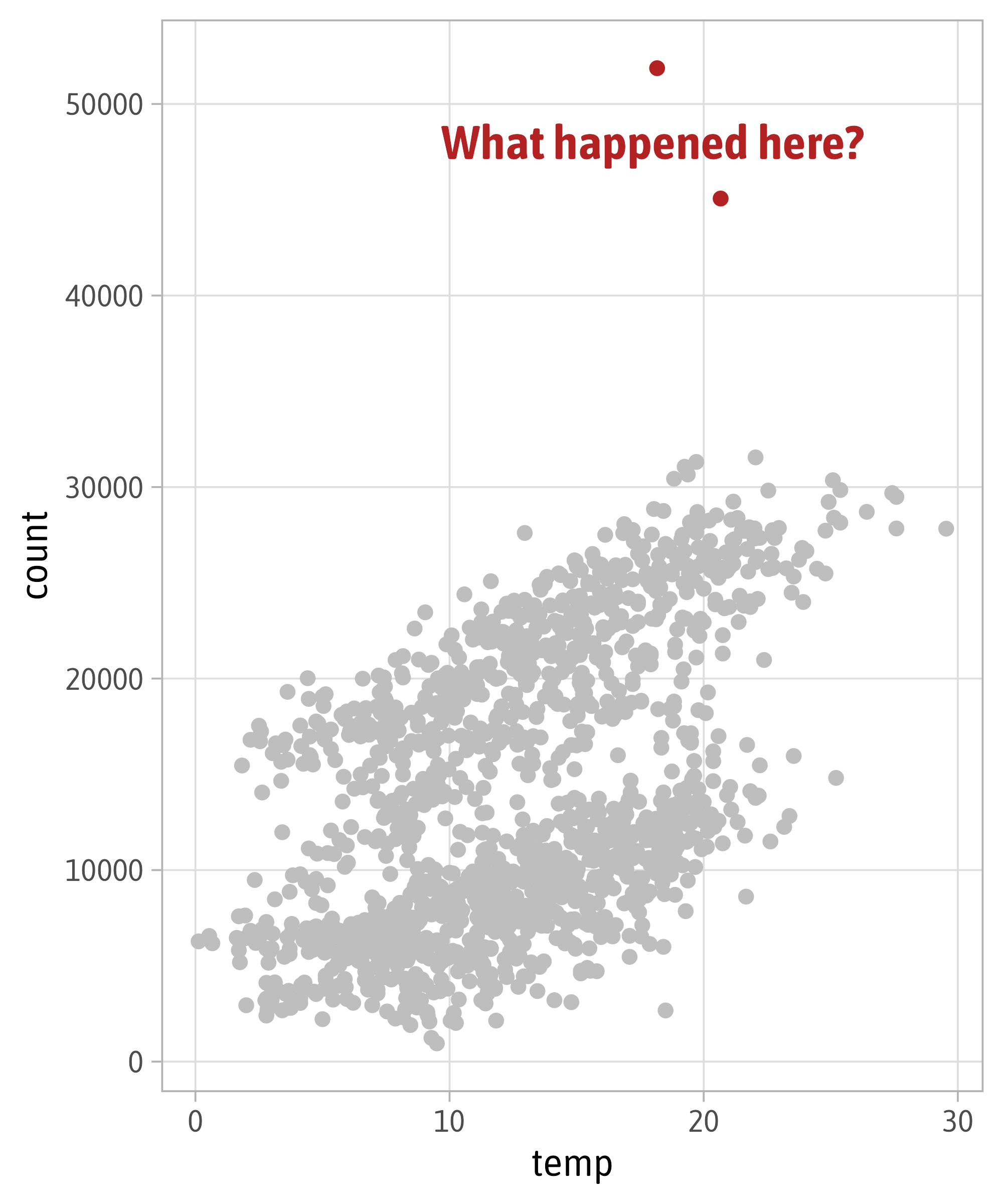
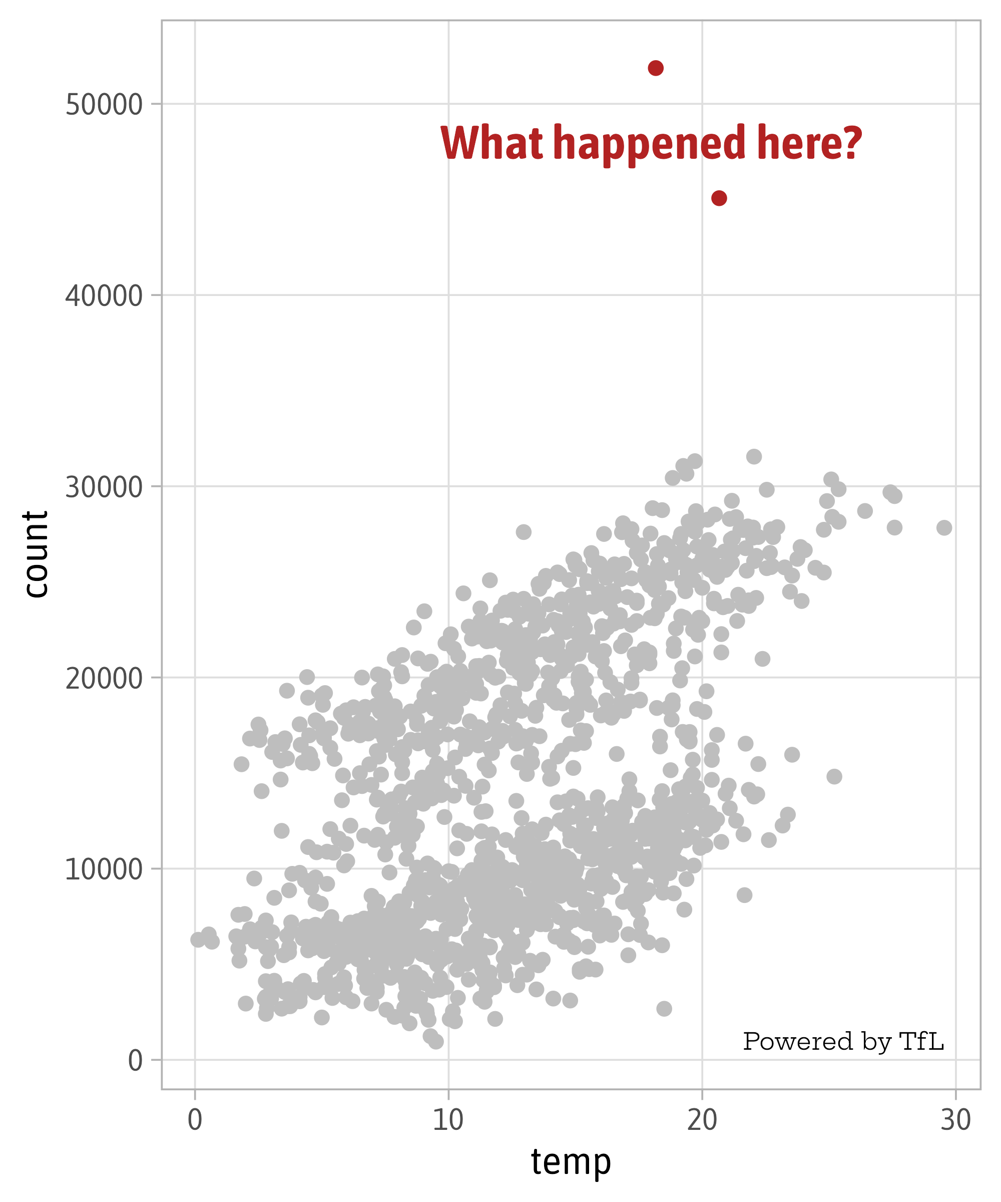
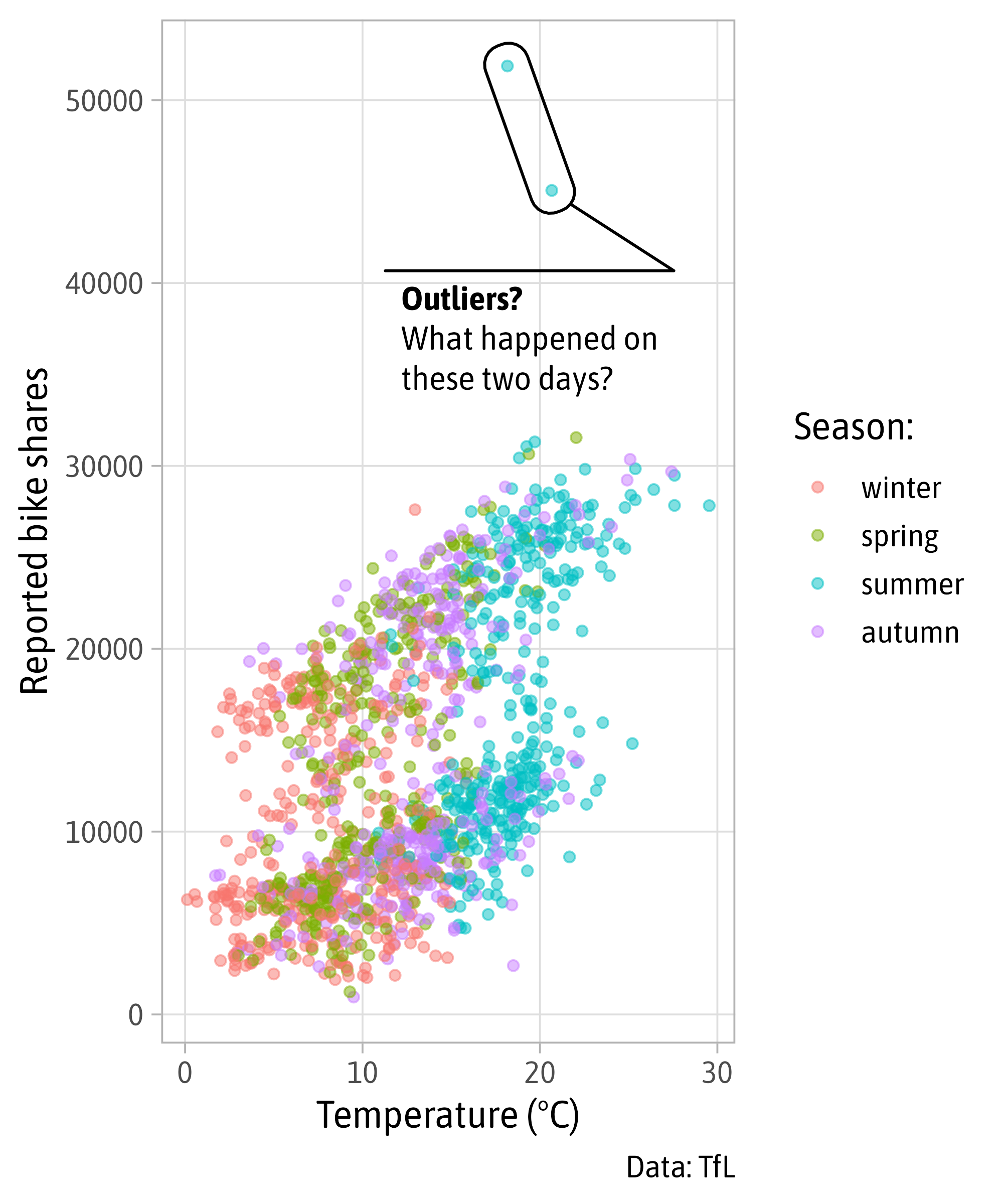
What happened on these<br>two <b style='color:#F7B01B;'>summer days</b>?
Styling Labels with {ggtext}
g +
  ggtext::geom_richtext(
    aes(x = 18, y = 48500,
        label = "What happened on these<br>two <b style='color:#F7B01B;'>summer days</b>?"),
    stat = "unique",
    color = "grey20",
    family = "Asap SemiCondensed",
    fill = NA,
    label.color = NA
  ) +
  scale_color_manual(
    values = c("#6681FE", "#1EC98D", "#F7B01B", "#A26E7C")
  )
What happened on these<br>two <b style='color:#F7B01B;'>summer days</b>?
Styling Labels with {ggtext}

Facet Labellers
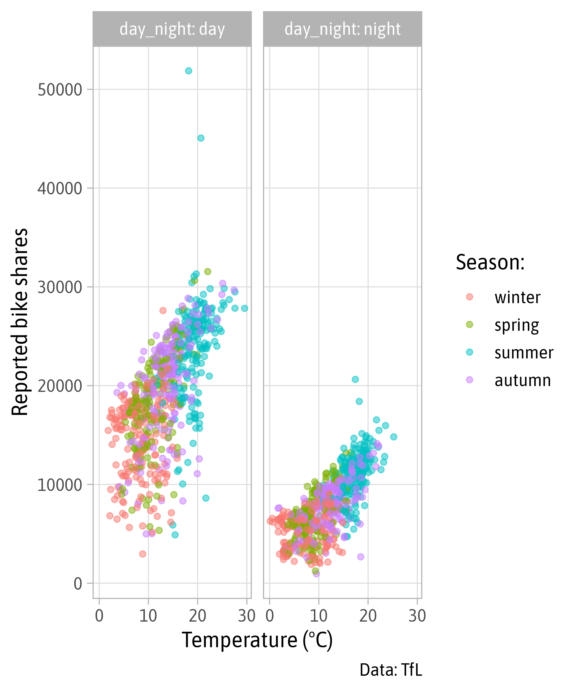
Facet Labellers
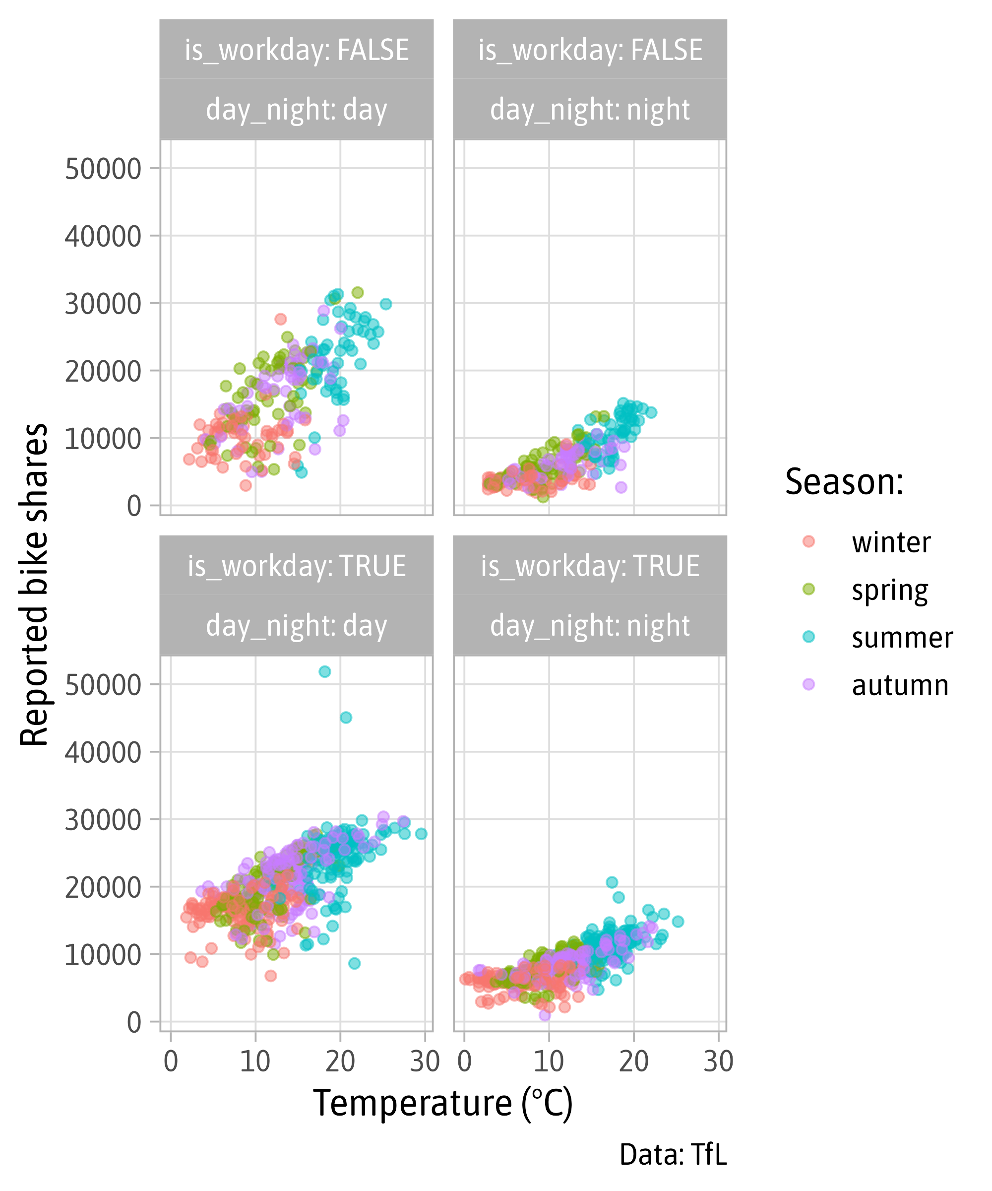
Facet Labellers

Facet Labellers

Facet Labellers
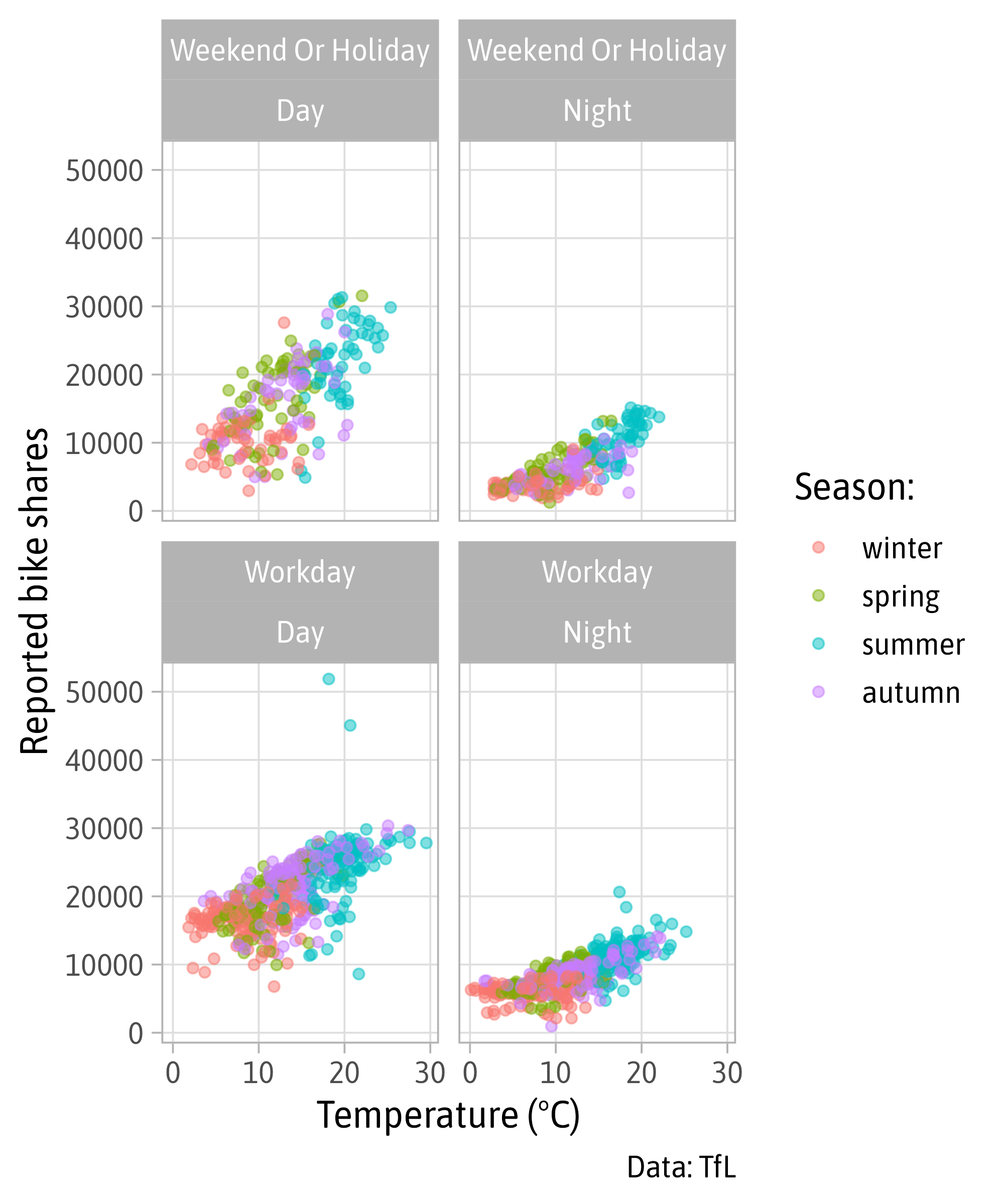
Facet Labeller
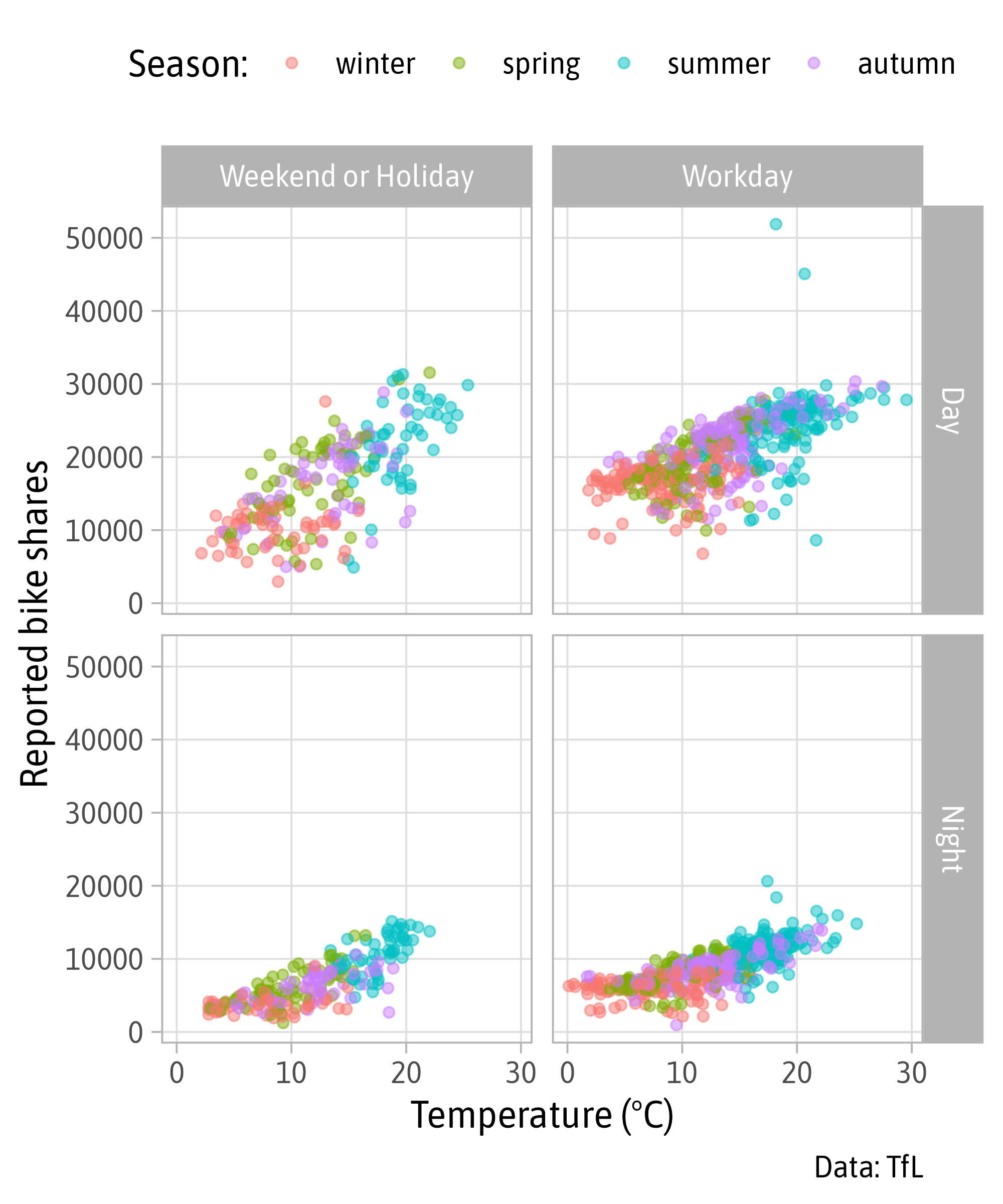
Handling Long Labels
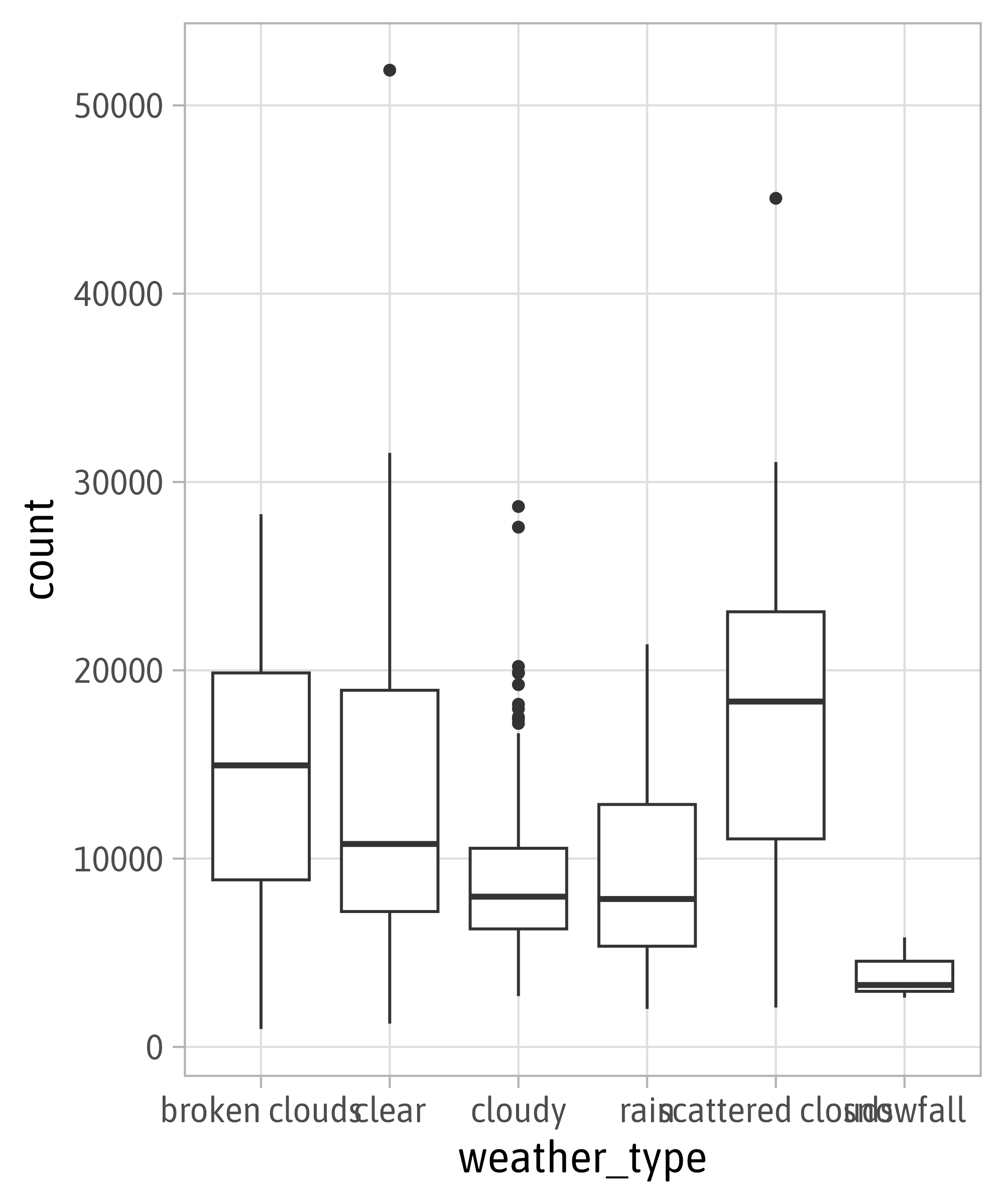
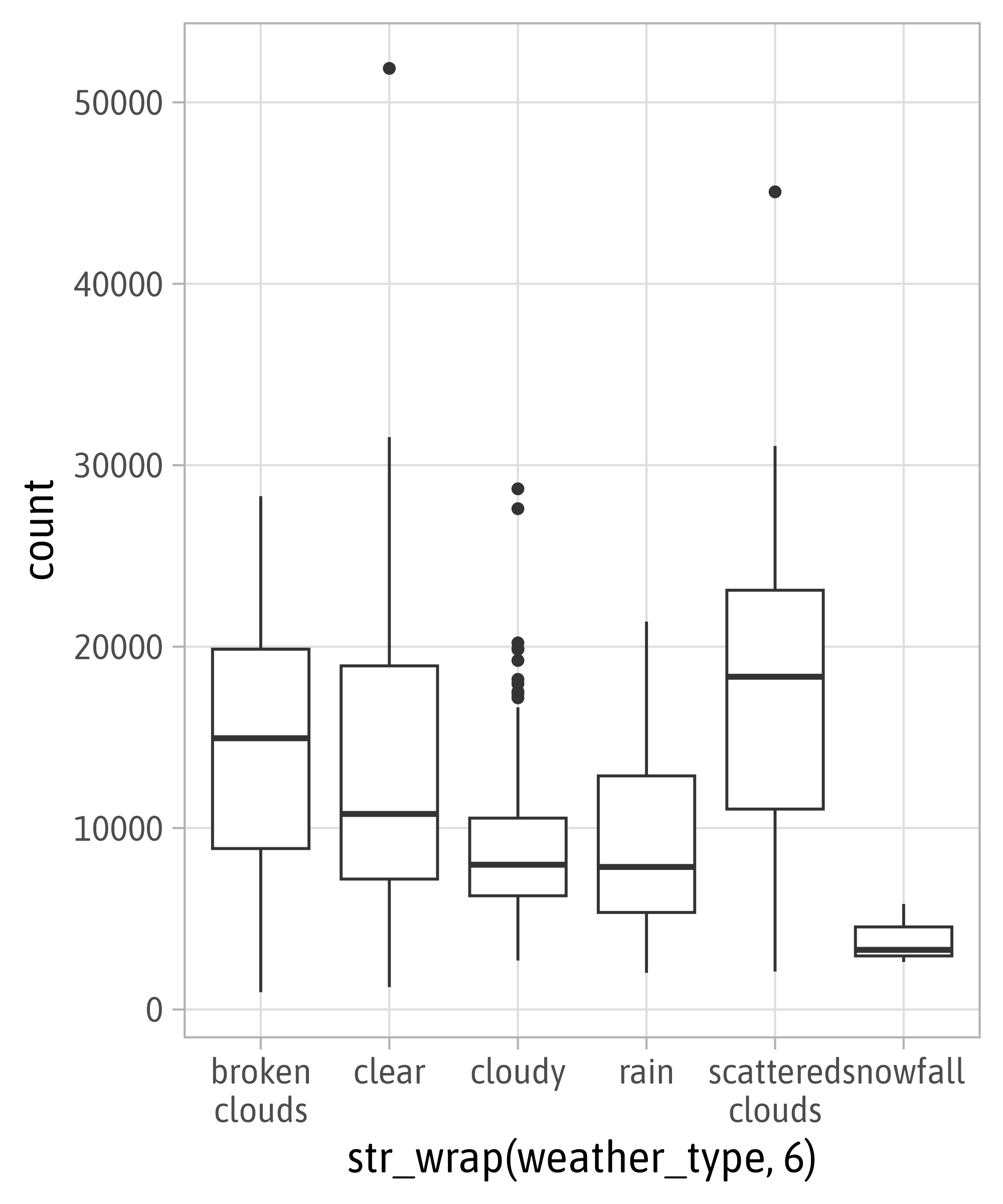
Handling Long Labels with {stringr}
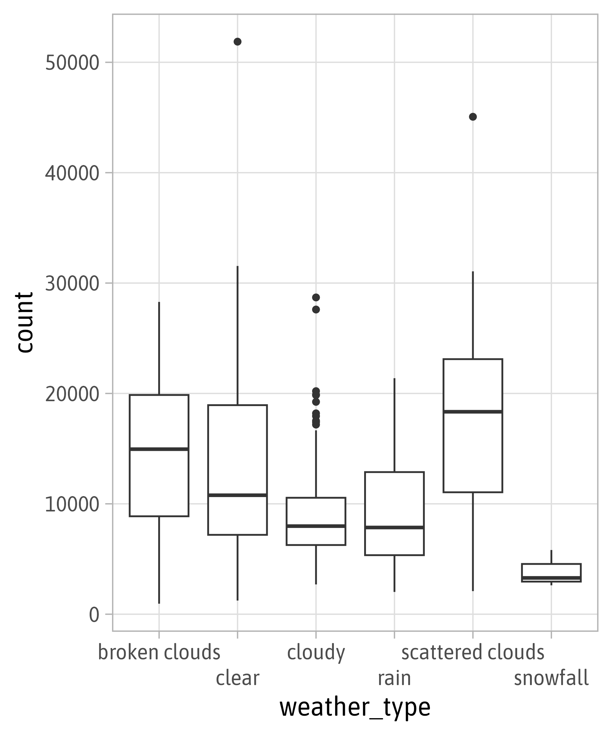
Handling Long Labels with {stringr}
Handling Long Titles
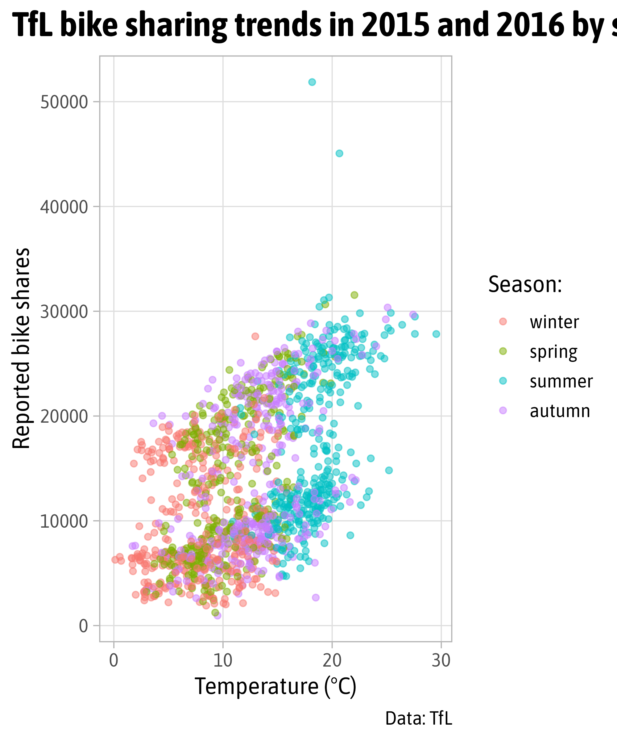
Handling Long Titles with
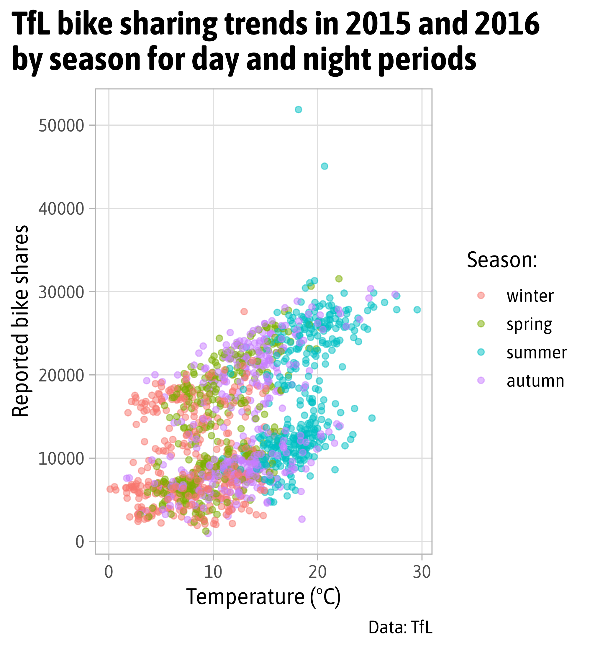
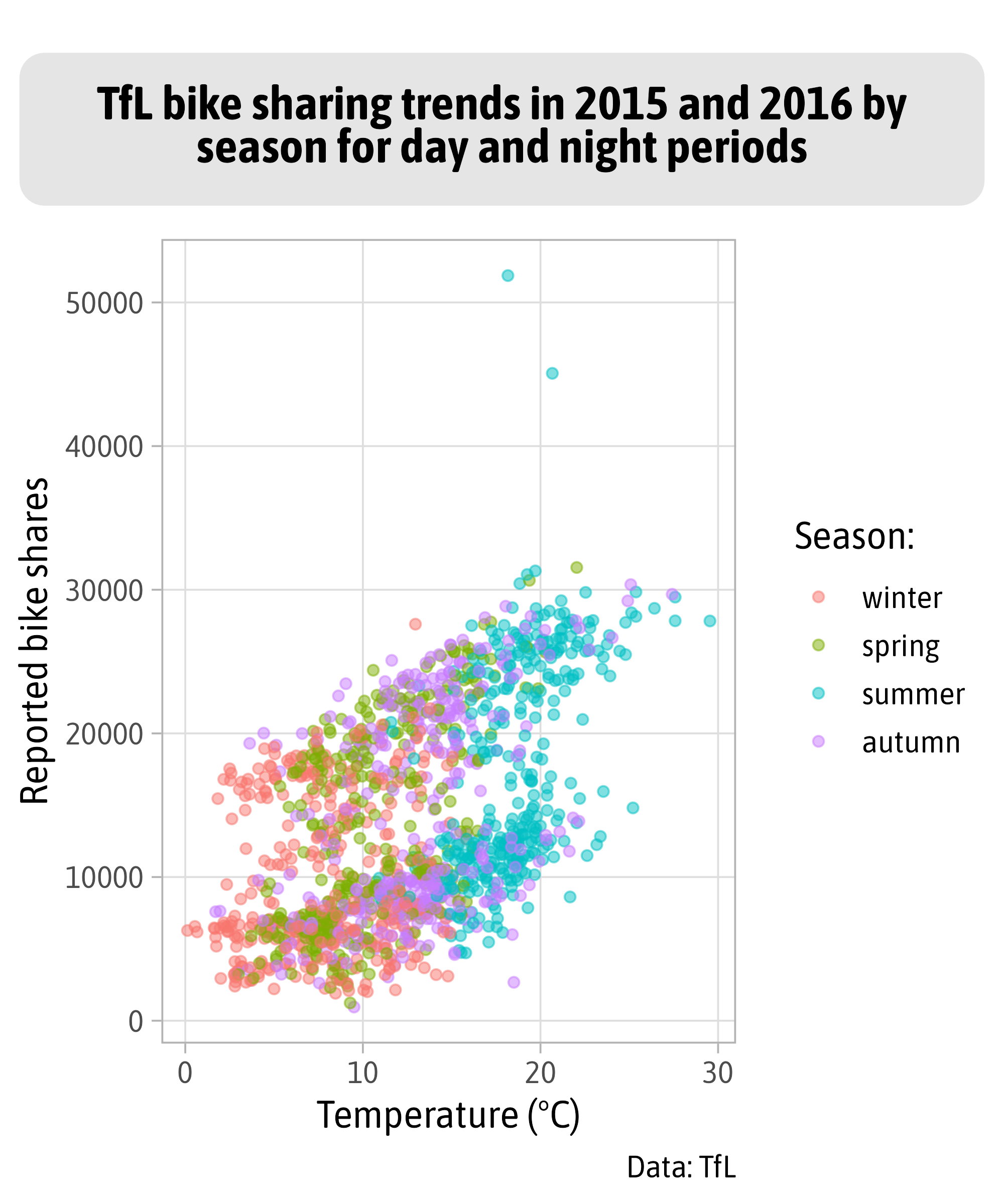
TfL bike sharing trends in 2015 and 2016\nby season for day and night periods
Handling Long Titles with {ggtext}
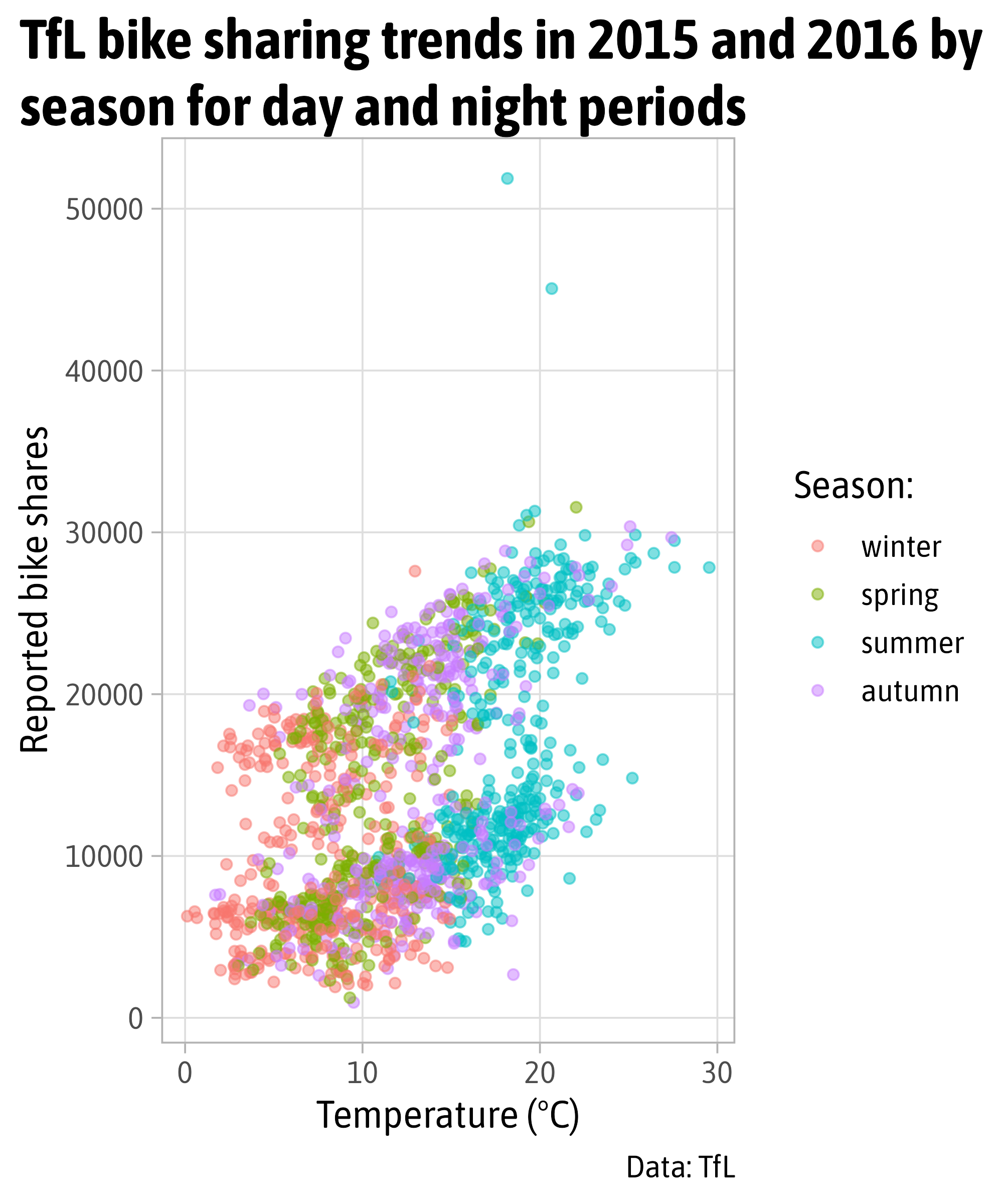
Handling Long Titles with {ggtext}
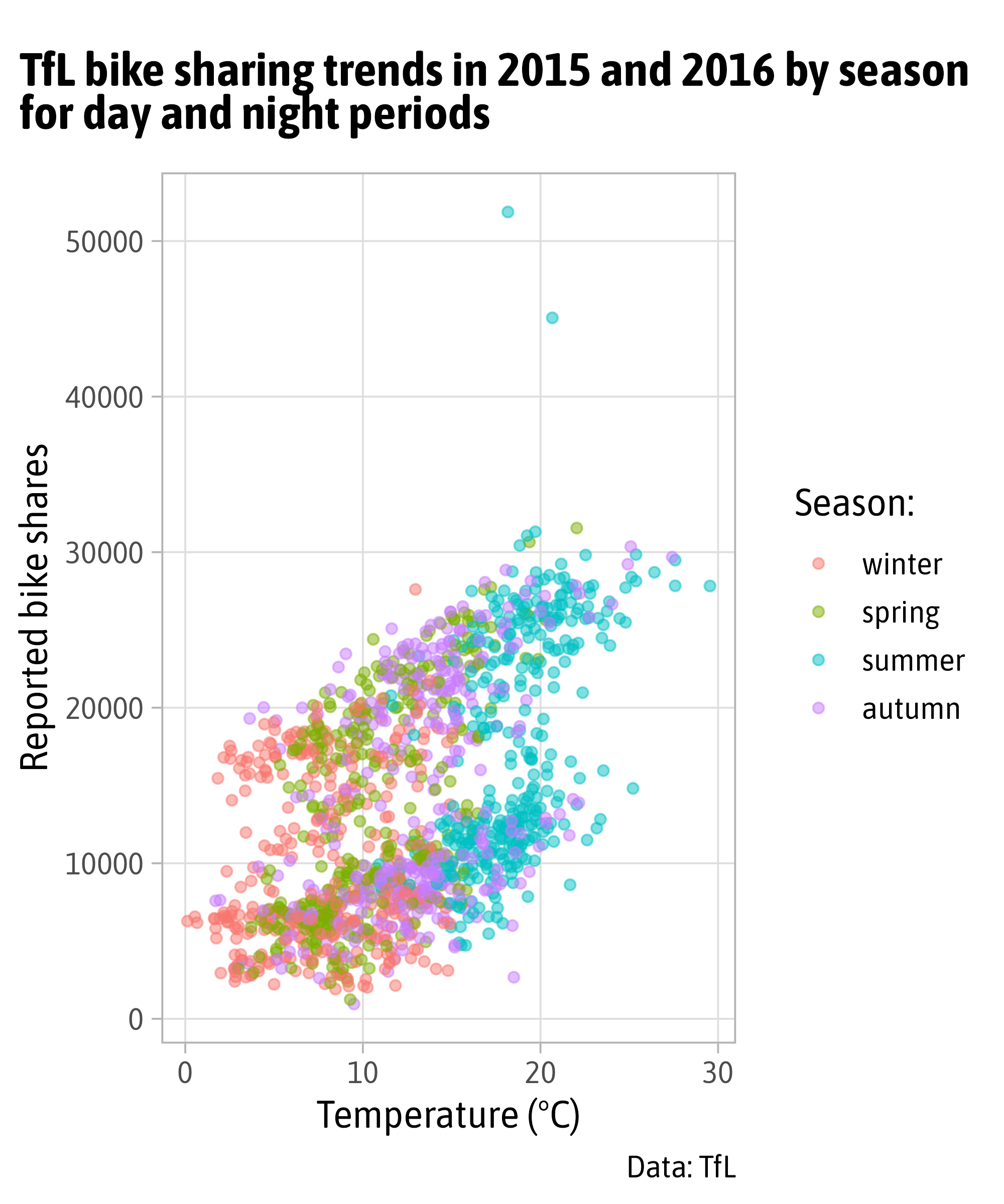
Handling Long Titles with {ggtext}
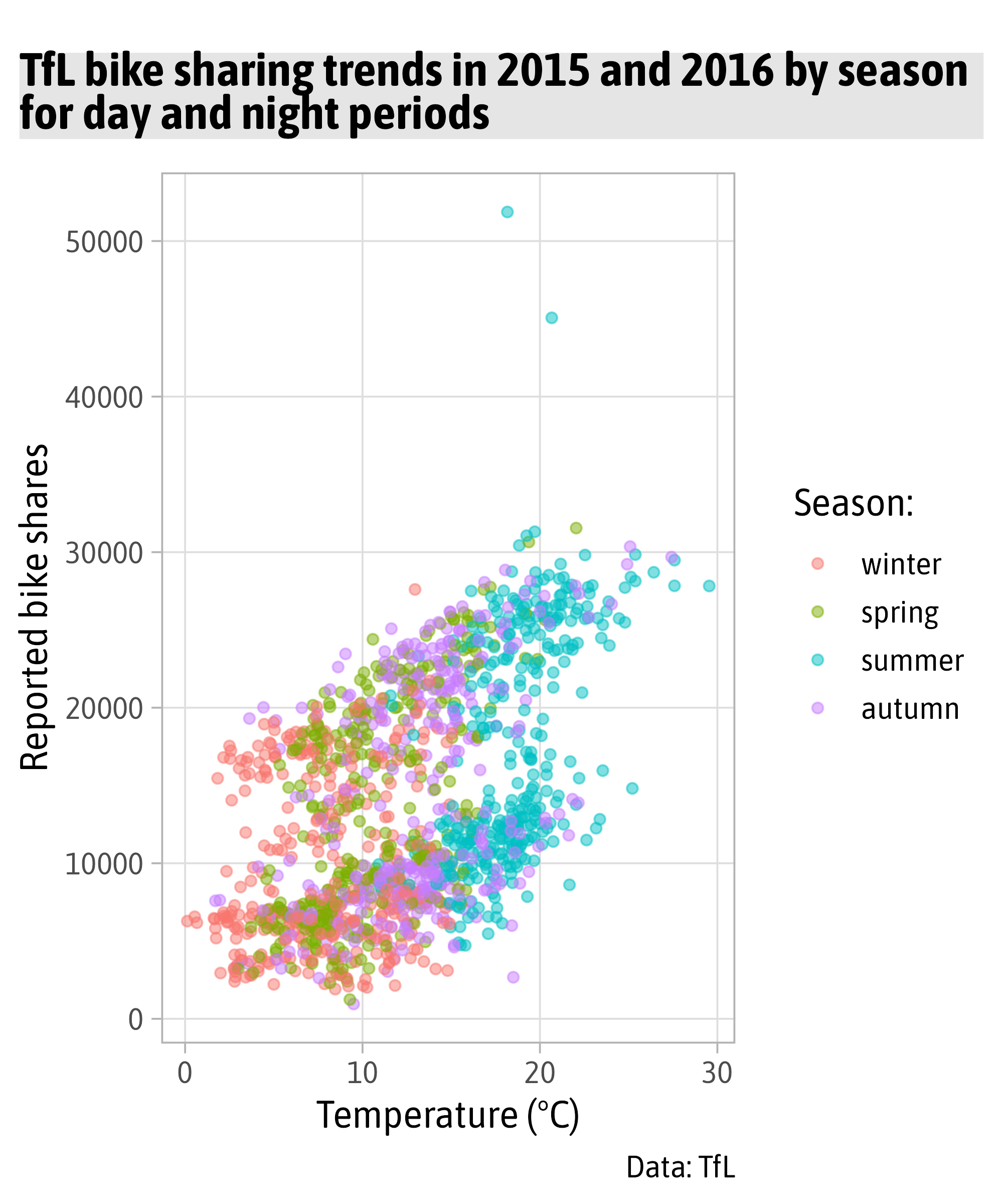
Handling Long Titles with {ggtext}
g +
  ggtitle("TfL bike sharing trends in 2015 and 2016 by season for day and night periods") +
  theme(
    plot.title = ggtext::element_textbox_simple(
      margin = margin(t = 12, b = 12),
      padding = margin(rep(12, 4)),
      fill = "grey90",
      box.color = "grey40",
      r = unit(9, "pt"),
      halign = .5,
      face = "bold",
      lineheight = .9
    ),
    plot.title.position = "plot"
  )
Add Single Text Annotations
Add Single Text Annotations
Style Text Annotations
Add Multiple Text Annotations
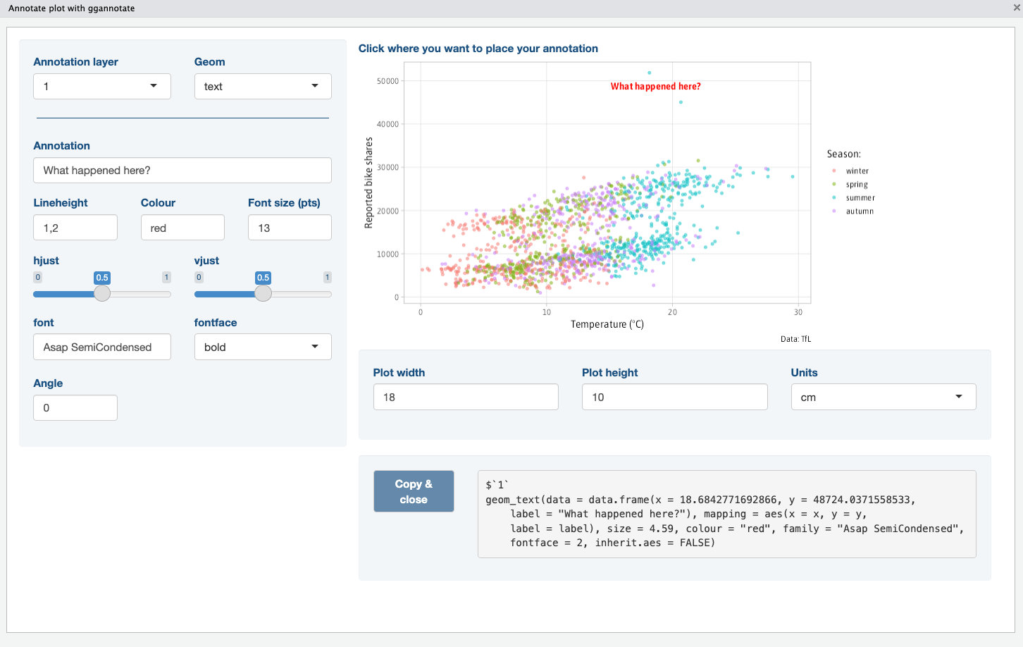
“Point’n’Click” Annotations
Add Boxes
Add Lines
Add Lines
Add Arrows
Add Arrows
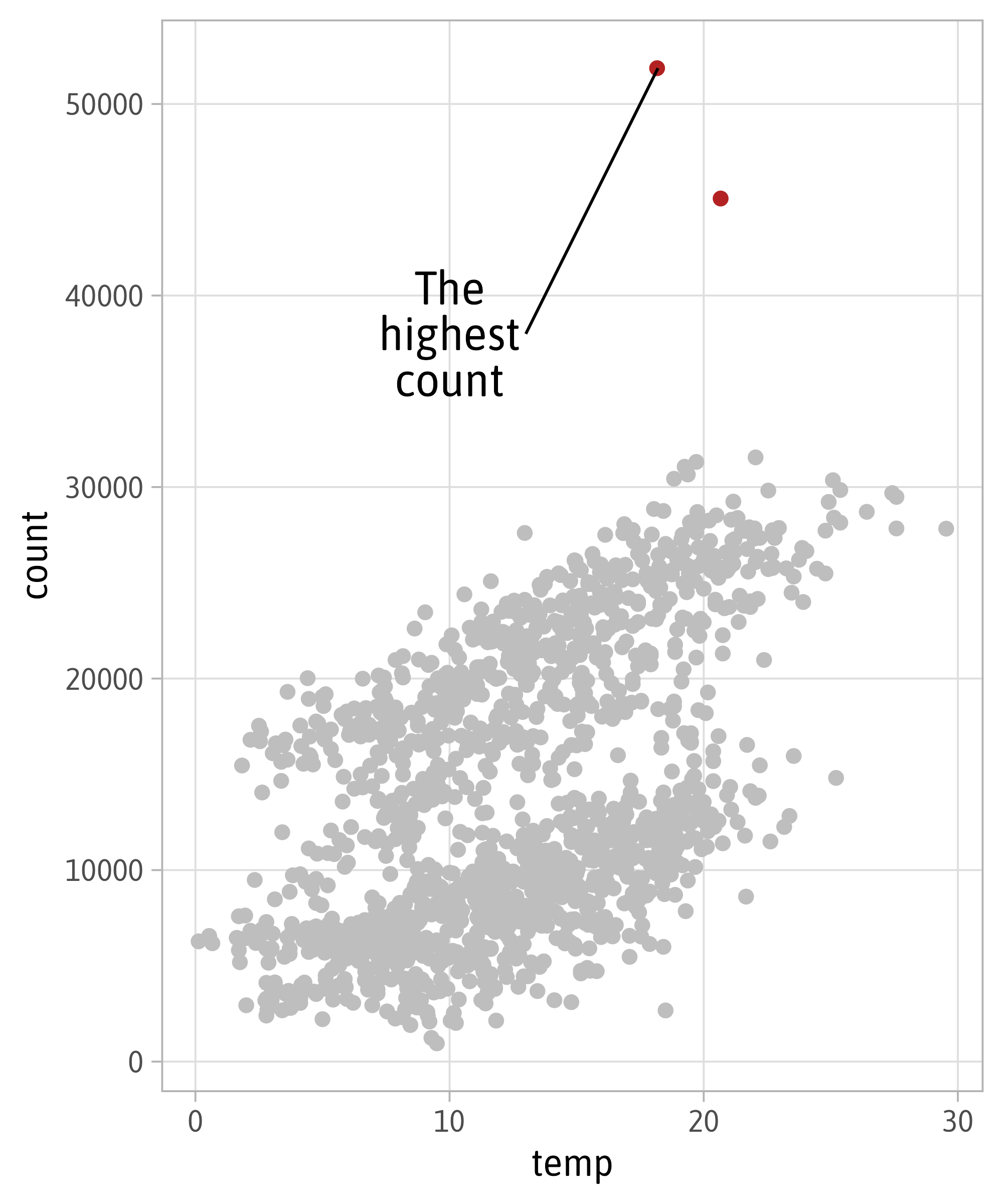
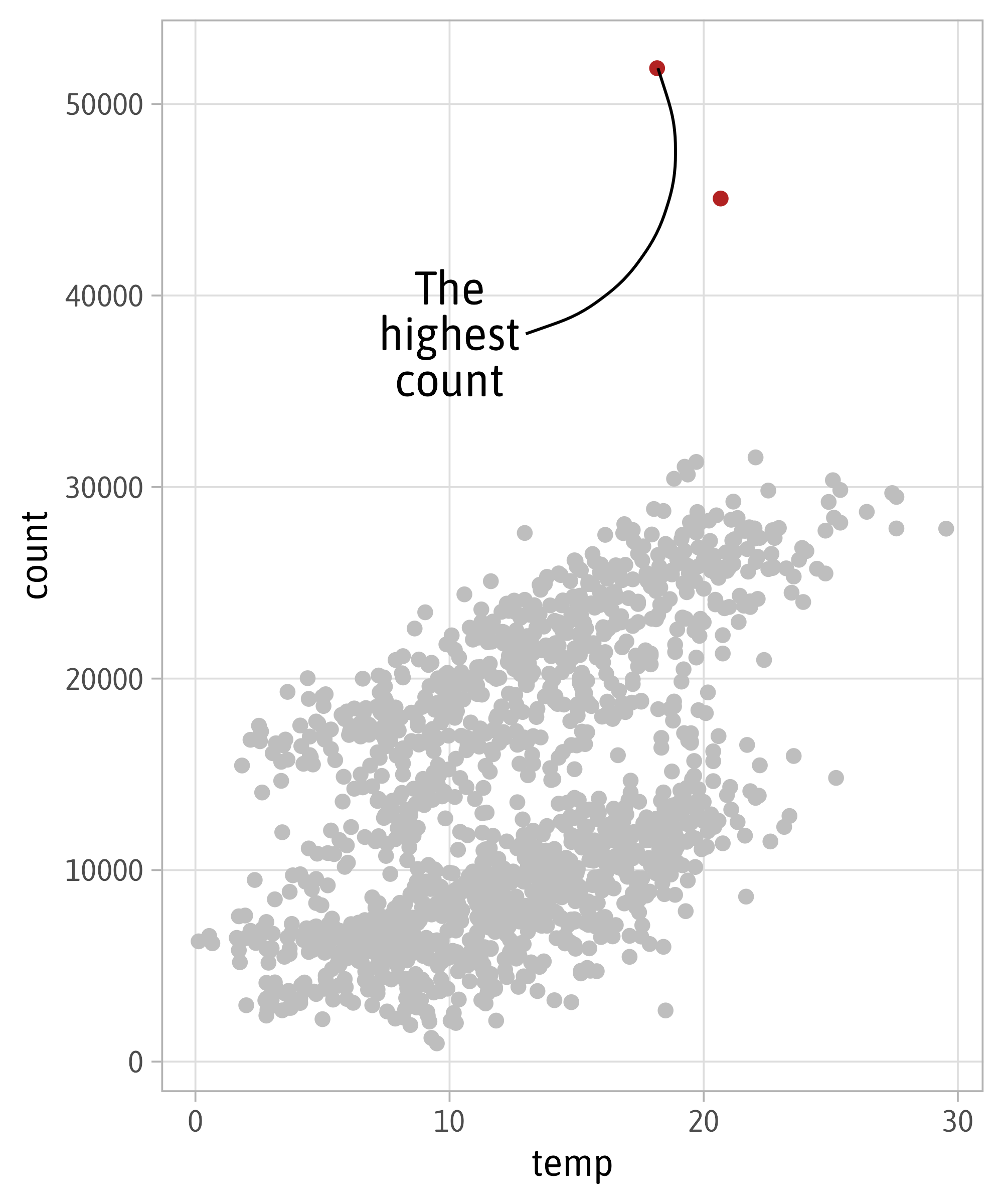
ga +
  annotate(
    geom = "text",
    x = 10,
    y = 38000,
    label = "The\nhighest\ncount",
    family = "Asap SemiCondensed",
    size = 6,
    lineheight =  .8
  ) +
  annotate(
    geom = "curve",
    x = 13,
    xend = 18.2,
    y = 38000,
    yend = 51870,
    curvature = .25,
    arrow = arrow(
      length = unit(10, "pt"),
      type = "closed",
      ends = "both"
    )
)![]()
Add Arrows
ga +
  annotate(
    geom = "text",
    x = 10,
    y = 38000,
    label = "The\nhighest\ncount",
    family = "Asap SemiCondensed",
    size = 6,
    lineheight =  .8
  ) +
  annotate(
    geom = "curve",
    x = 13,
    xend = 18.2,
    y = 38000,
    yend = 51870,
    curvature = .8,
    angle = 130,
    arrow = arrow(
      length = unit(10, "pt"),
      type = "closed"
    )
)![]()
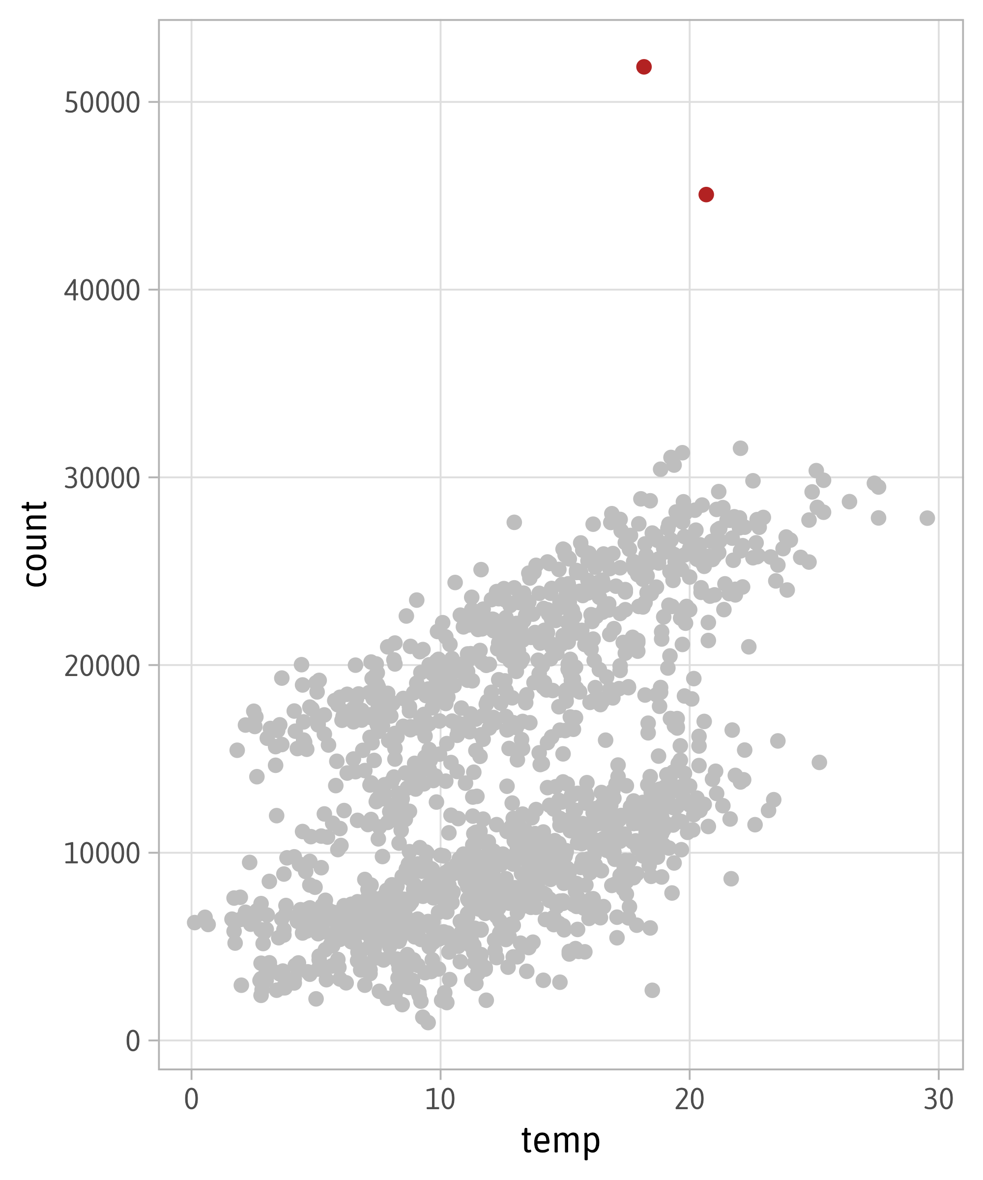
Highlight Hot Days
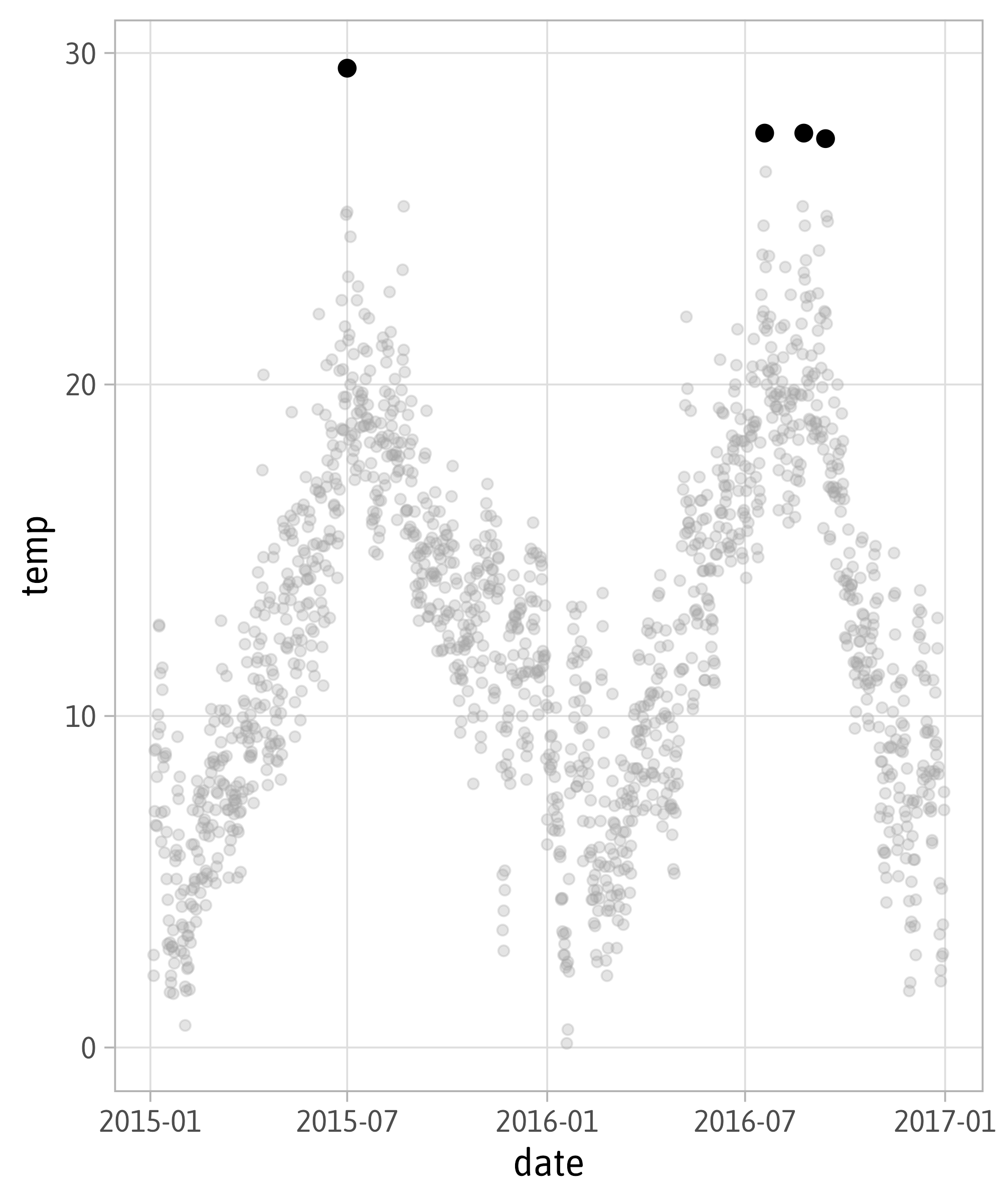
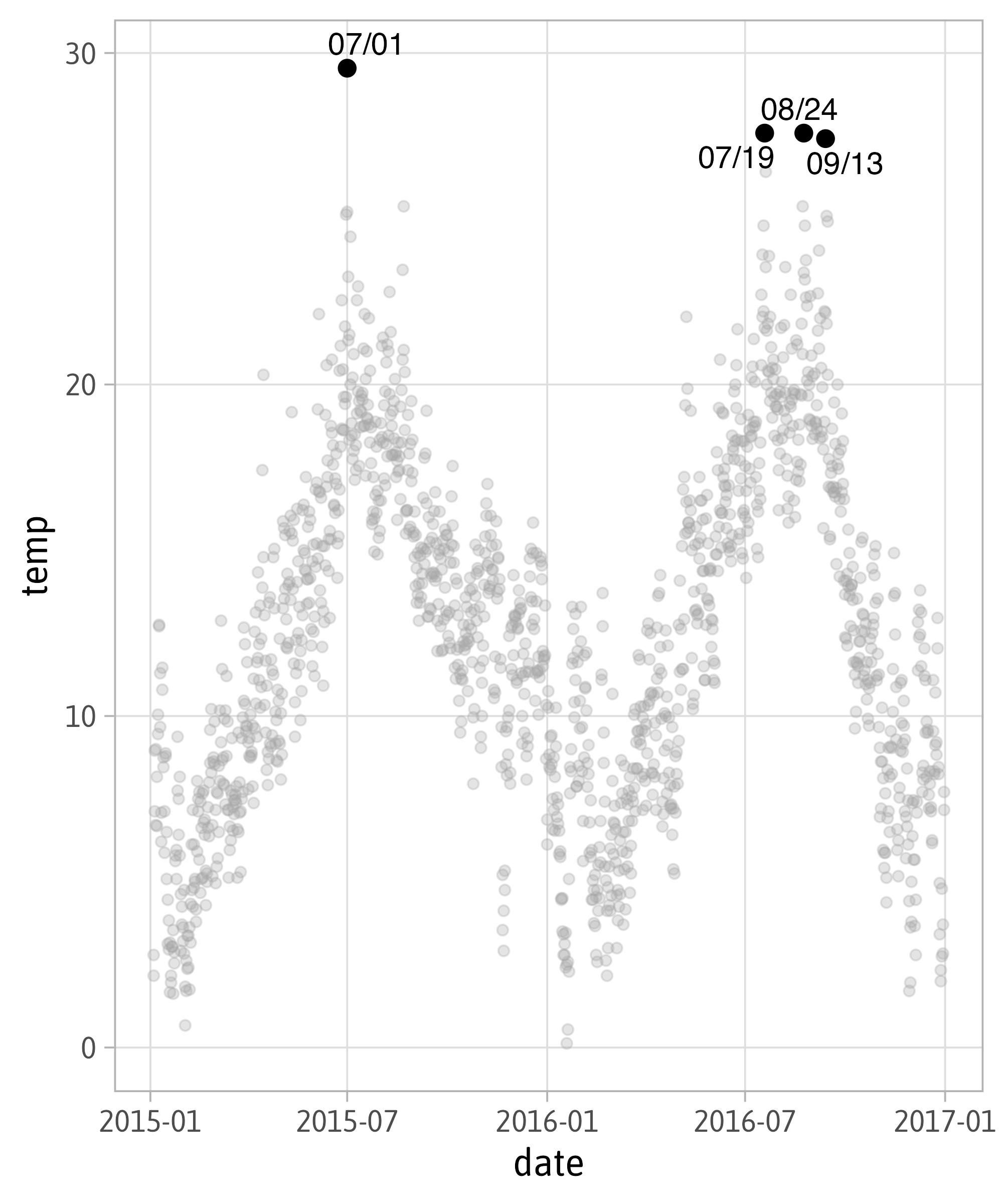
Annotations with geom_text()
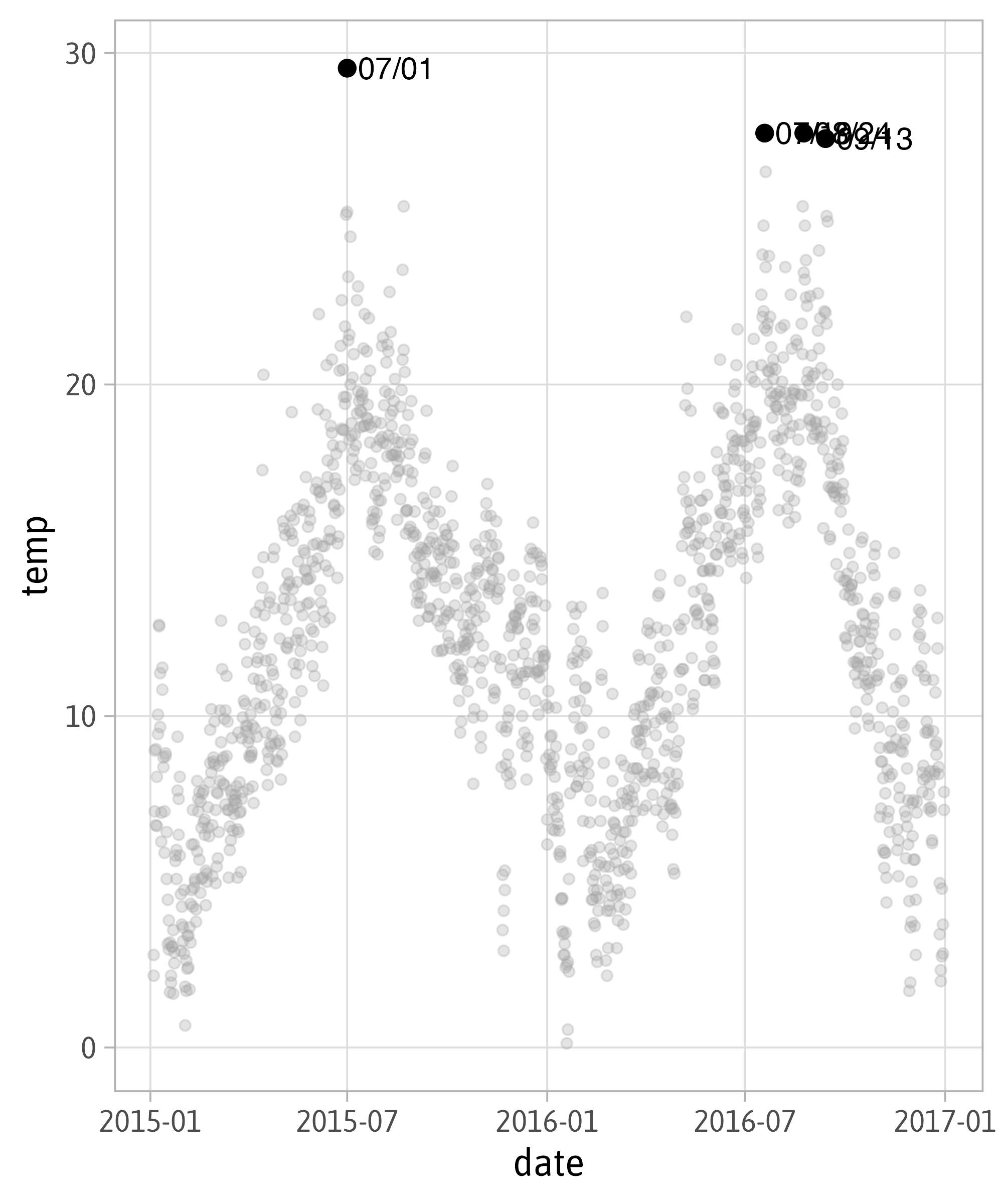
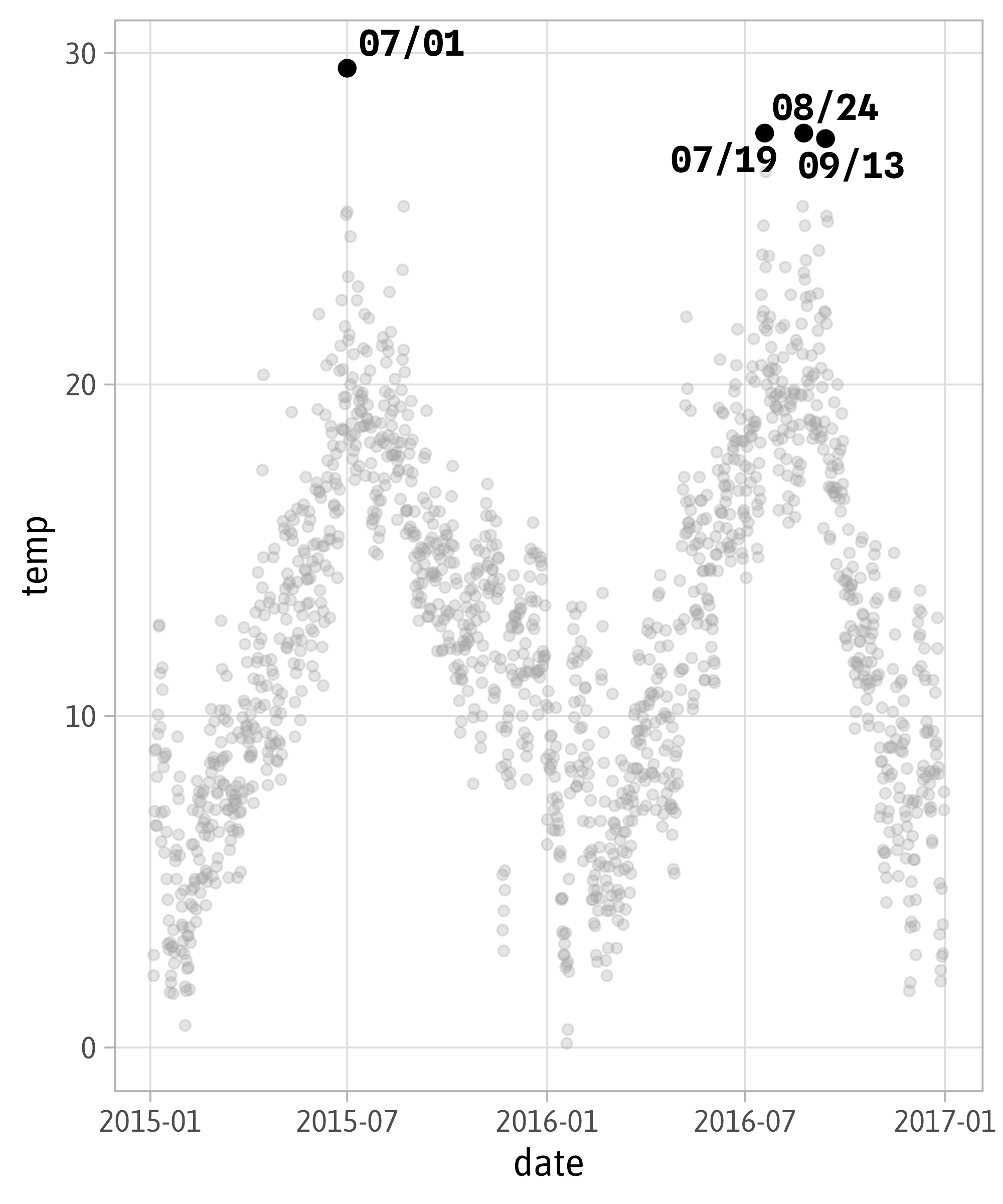
Annotations with geom_label()
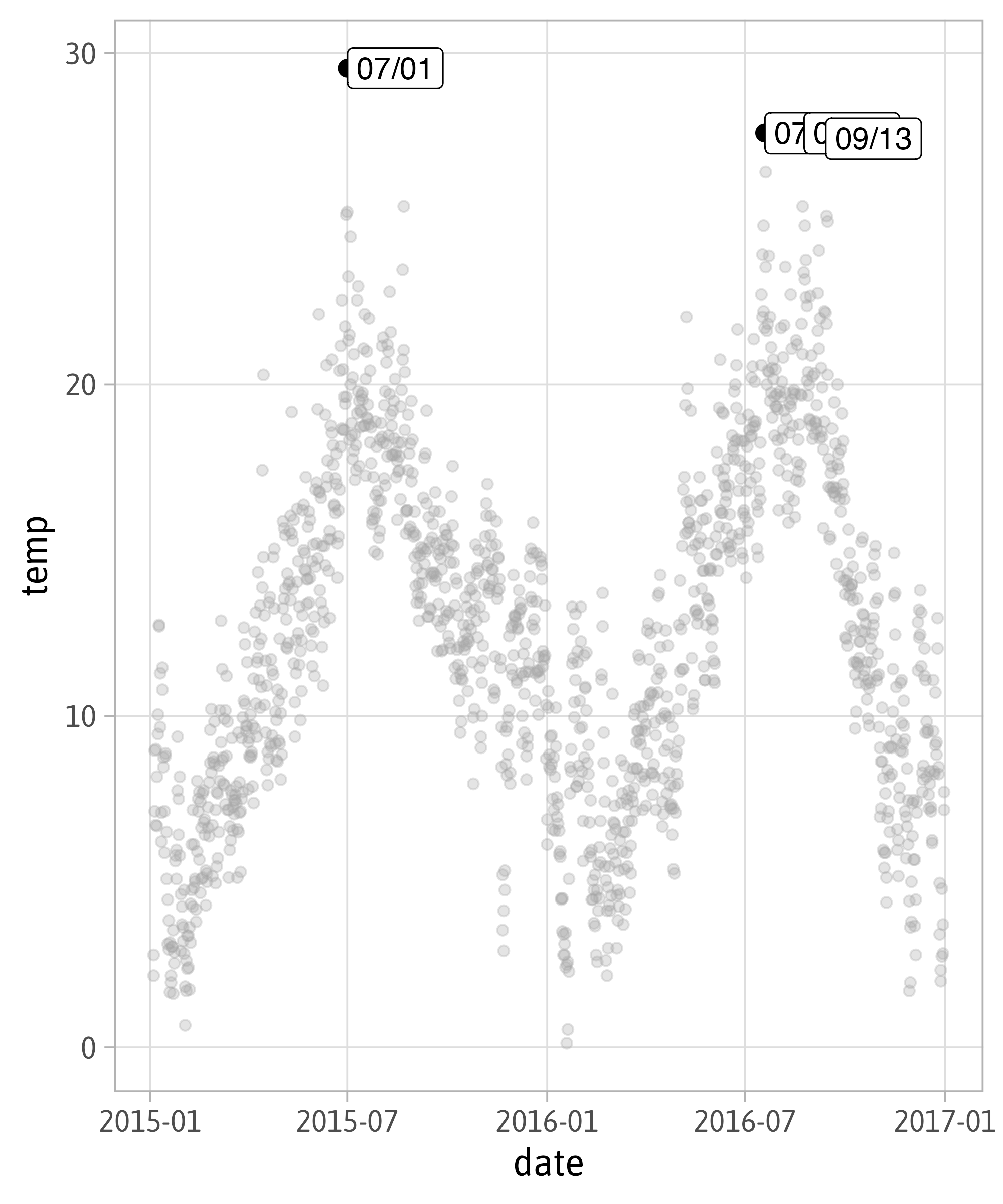
Annotations with {ggrepel}
Annotations with {ggrepel}
Annotations with {ggrepel}
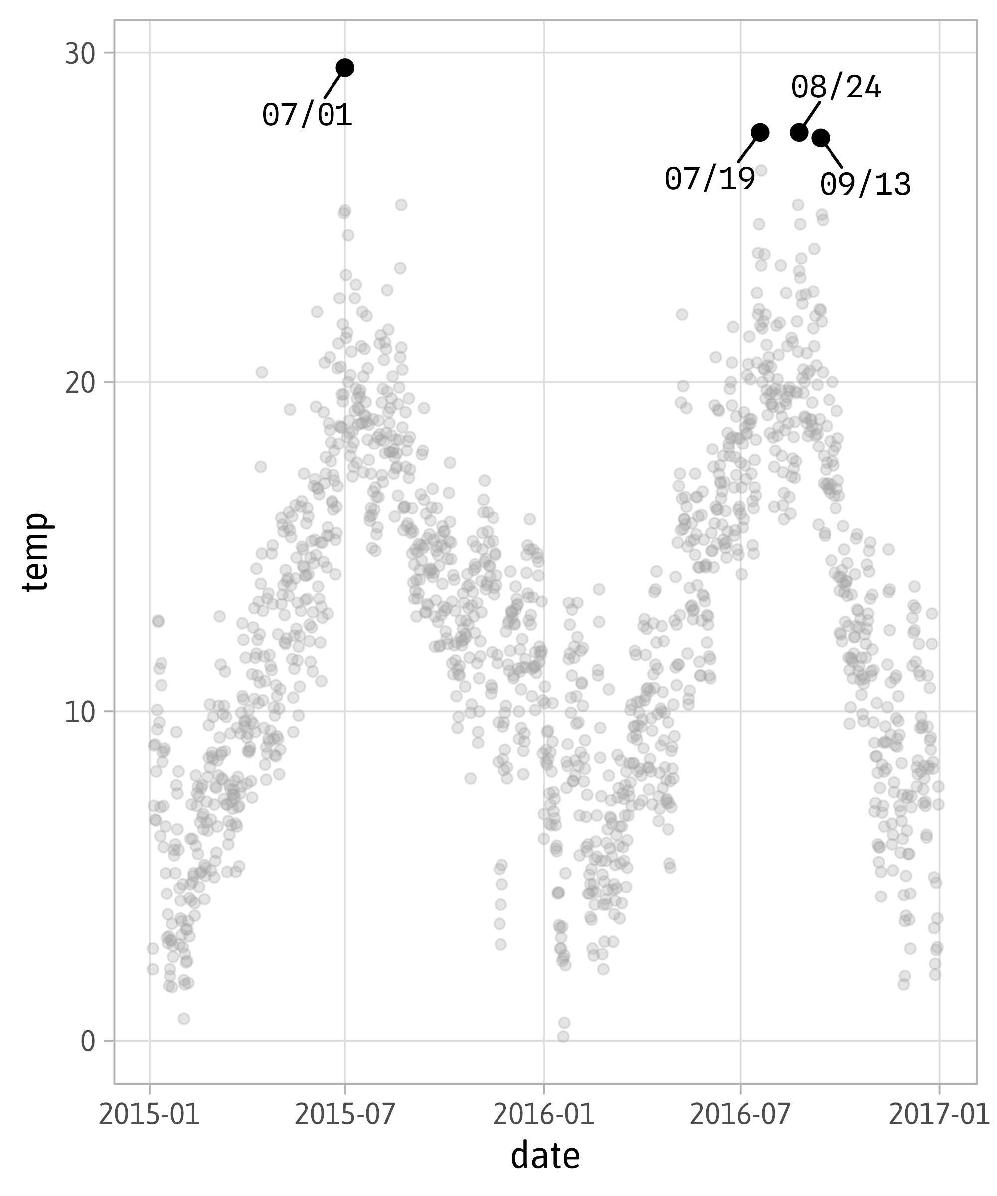
Annotations with {ggrepel}

Annotations with {ggrepel}
Annotations with {ggrepel}
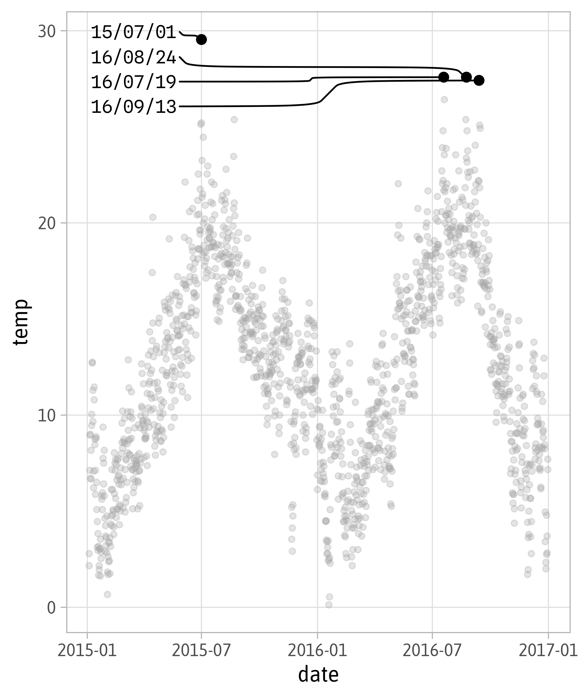
Annotations with {ggforce}
Annotations with {ggforce}
Annotations with {ggforce}
Annotations with {ggforce}
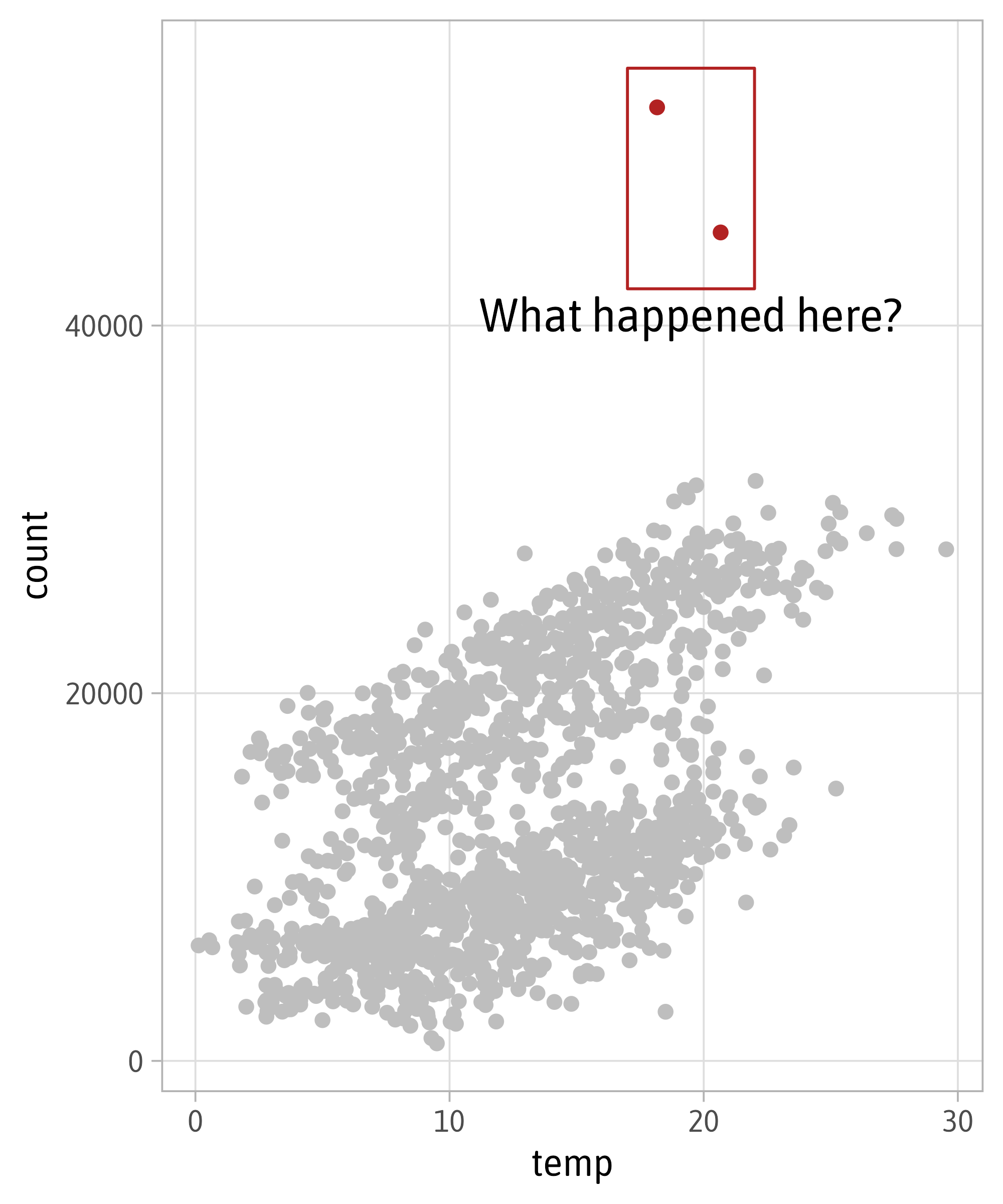
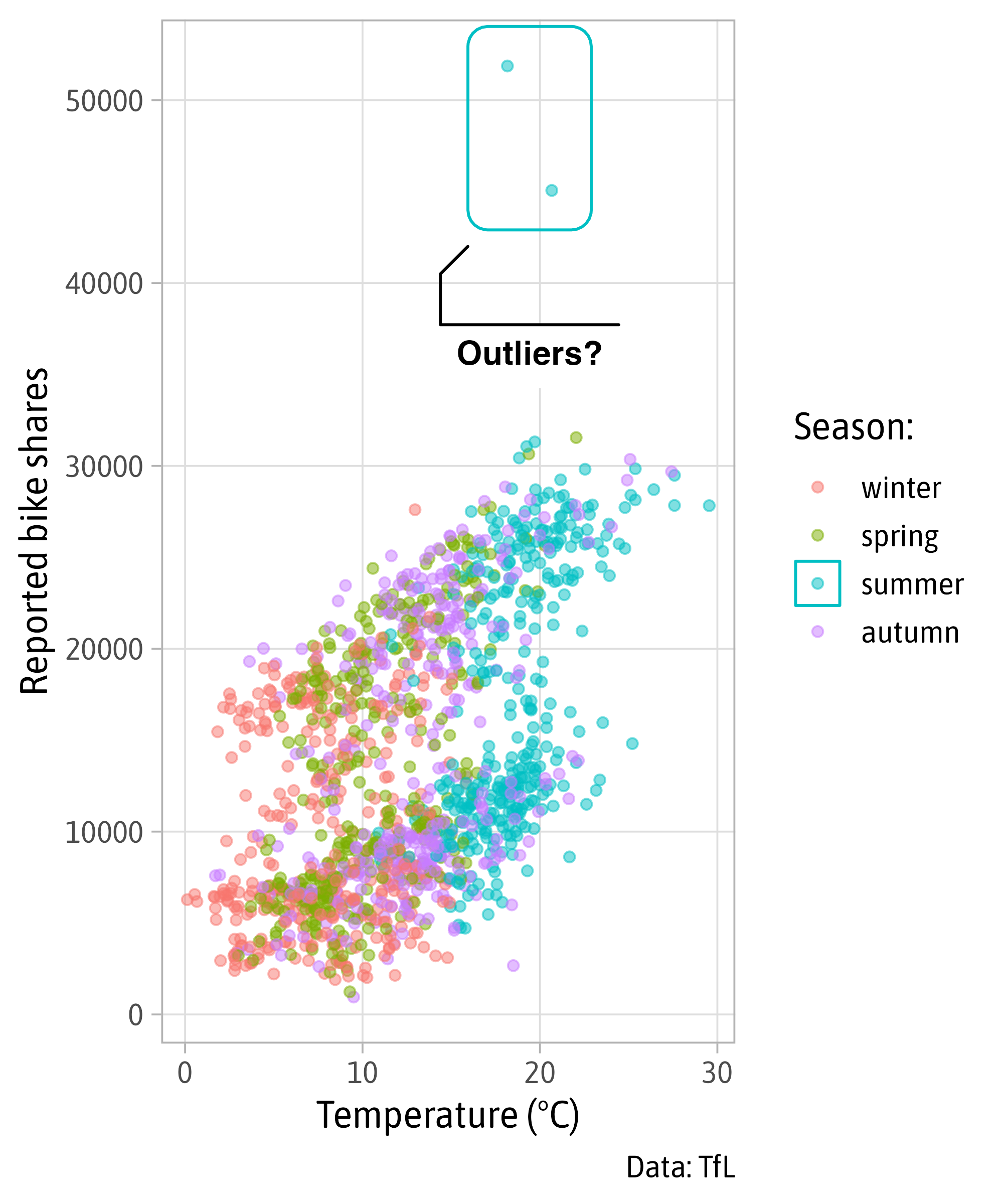
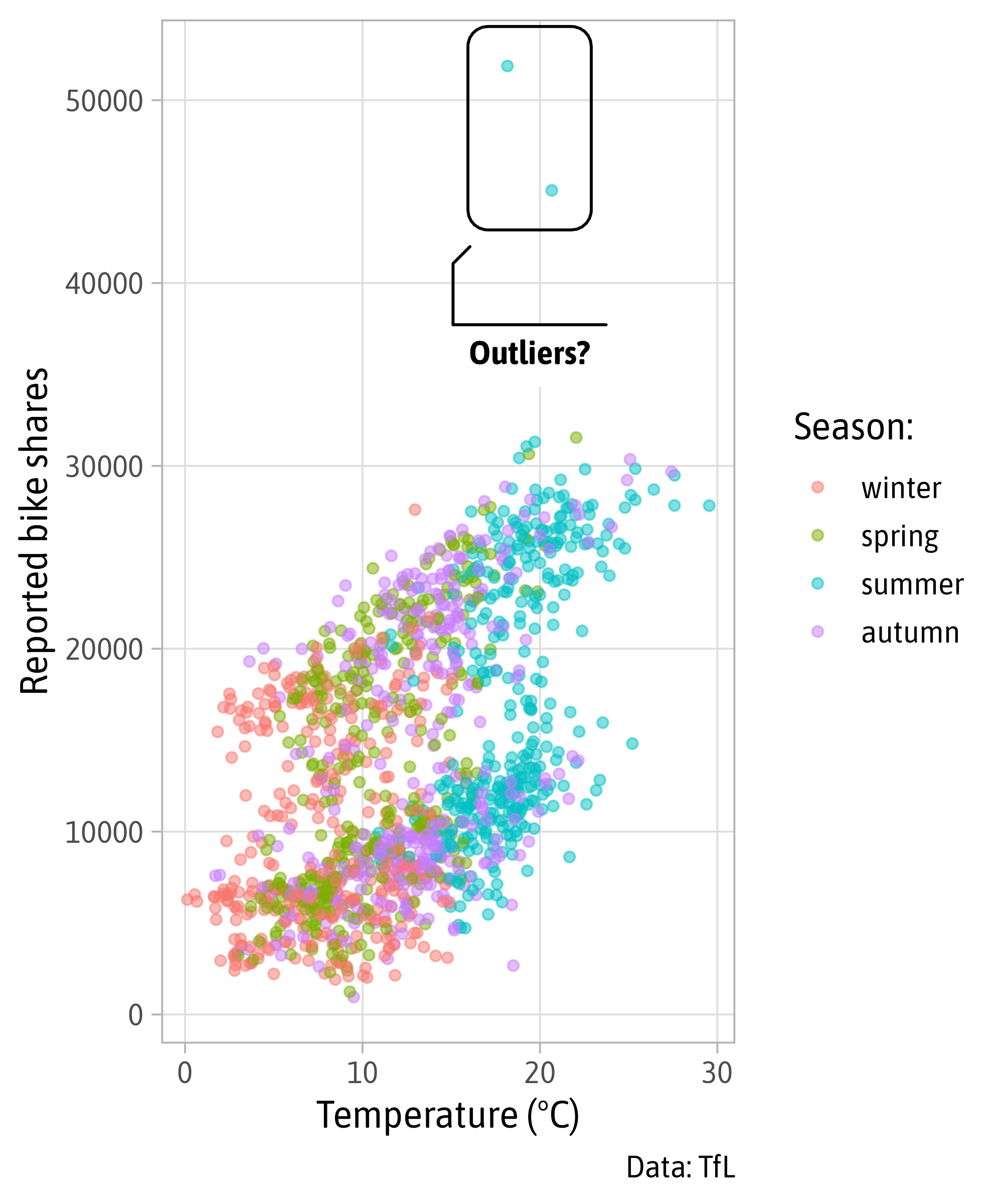
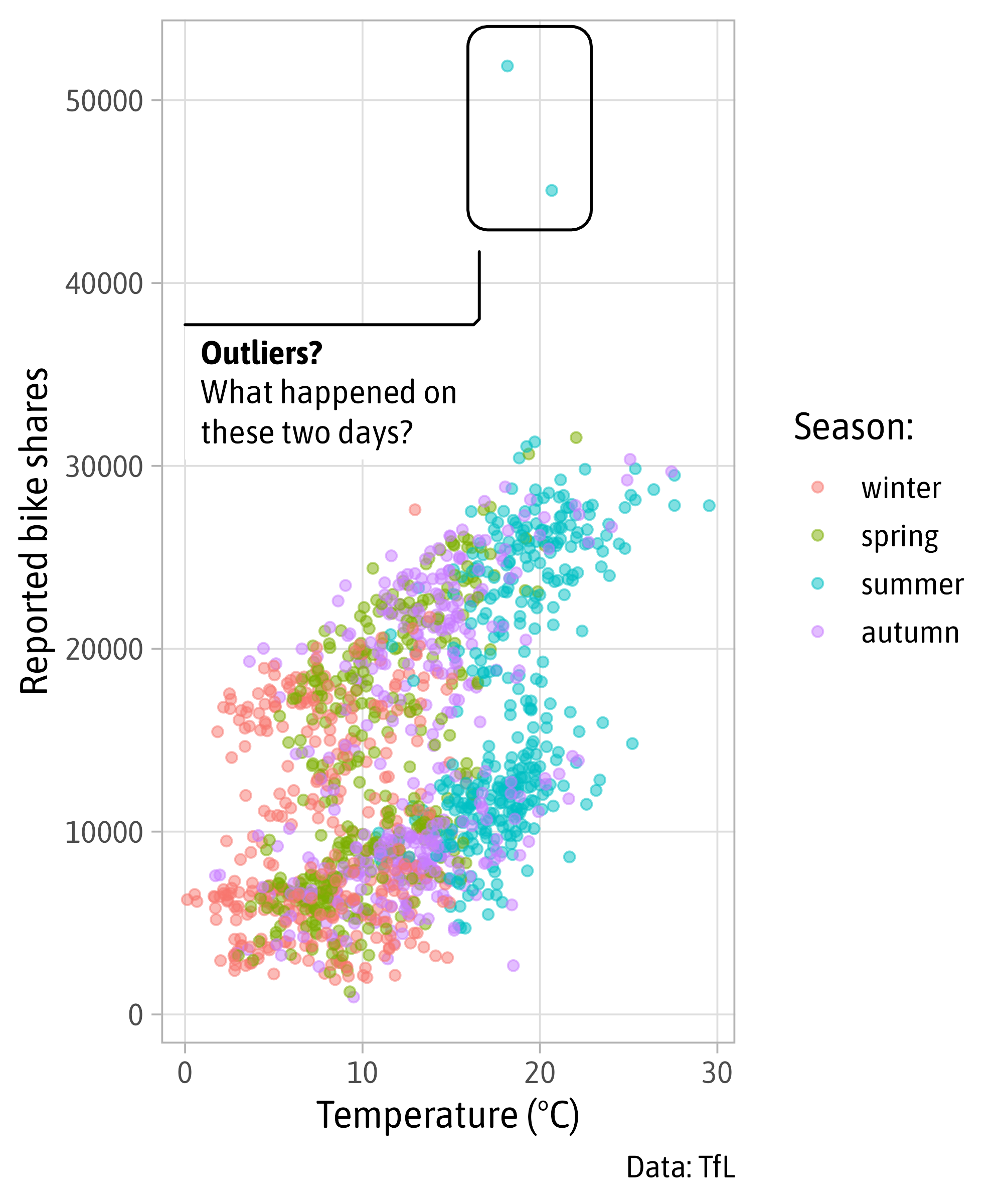
g +
  ggforce::geom_mark_rect(
    aes(label = "Outliers?",
        filter = count > 40000),
    description = "What happened on\nthese two days?",
    color = "black",
    label.family = "Asap SemiCondensed",
    expand = unit(8, "pt"),
    radius = unit(12, "pt"),
    con.cap = unit(0, "pt"),
    label.buffer = unit(15, "pt"),
    con.type = "straight",
    label.fill = "transparent"
  )
Annotations with {ggforce}
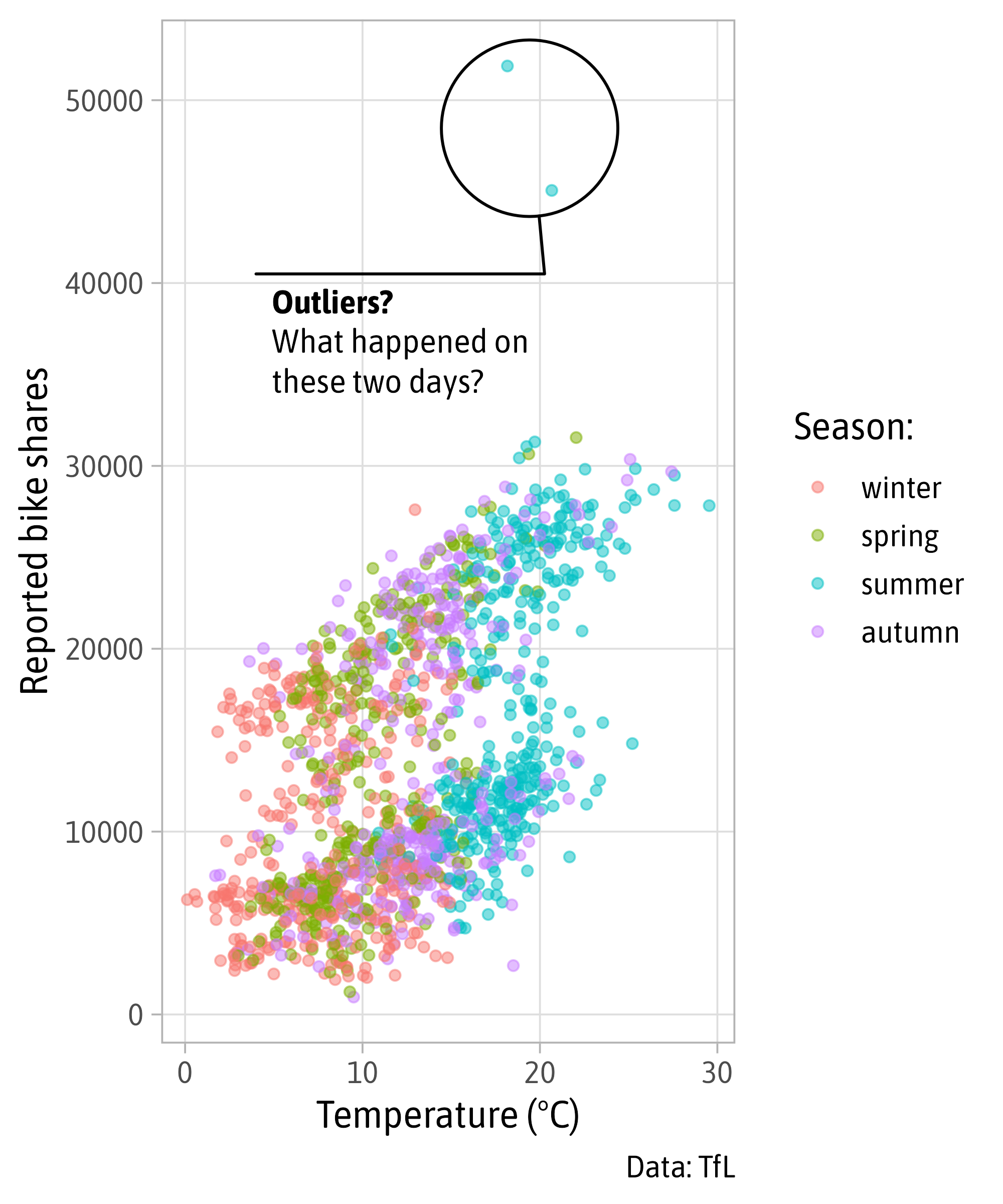
g +
  ggforce::geom_mark_circle(
    aes(label = "Outliers?",
        filter = count > 40000),
    description = "What happened on\nthese two days?",
    color = "black",
    label.family = "Asap SemiCondensed",
    expand = unit(8, "pt"),
    con.cap = unit(0, "pt"),
    label.buffer = unit(15, "pt"),
    con.type = "straight",
    label.fill = "transparent"
  )
Annotations with {ggforce}
g +
  ggforce::geom_mark_hull(
    aes(label = "Outliers?",
        filter = count > 40000),
    description = "What happened on\nthese two days?",
    color = "black",
    label.family = "Asap SemiCondensed",
    expand = unit(8, "pt"),
    con.cap = unit(0, "pt"),
    label.buffer = unit(15, "pt"),
    con.type = "straight",
    label.fill = "transparent"
  )
Annotations with {geomtextpath}
bikes |>
  filter(year == "2016") |>
  group_by(month, day_night) |>
  summarize(count = sum(count)) |>
  ggplot(aes(x = month, y = count,
             color = day_night,
             group = day_night)) +
  geom_line(linewidth = 1) +
  coord_cartesian(expand = FALSE) +
  scale_y_continuous(
    labels = scales::label_comma(
      scale = 1/10^3, suffix = "K"
    ),
    limits = c(0, 850000)
  ) +
  scale_color_manual(
    values = c("#FFA200", "#757BC7"),
    name = NULL
  )
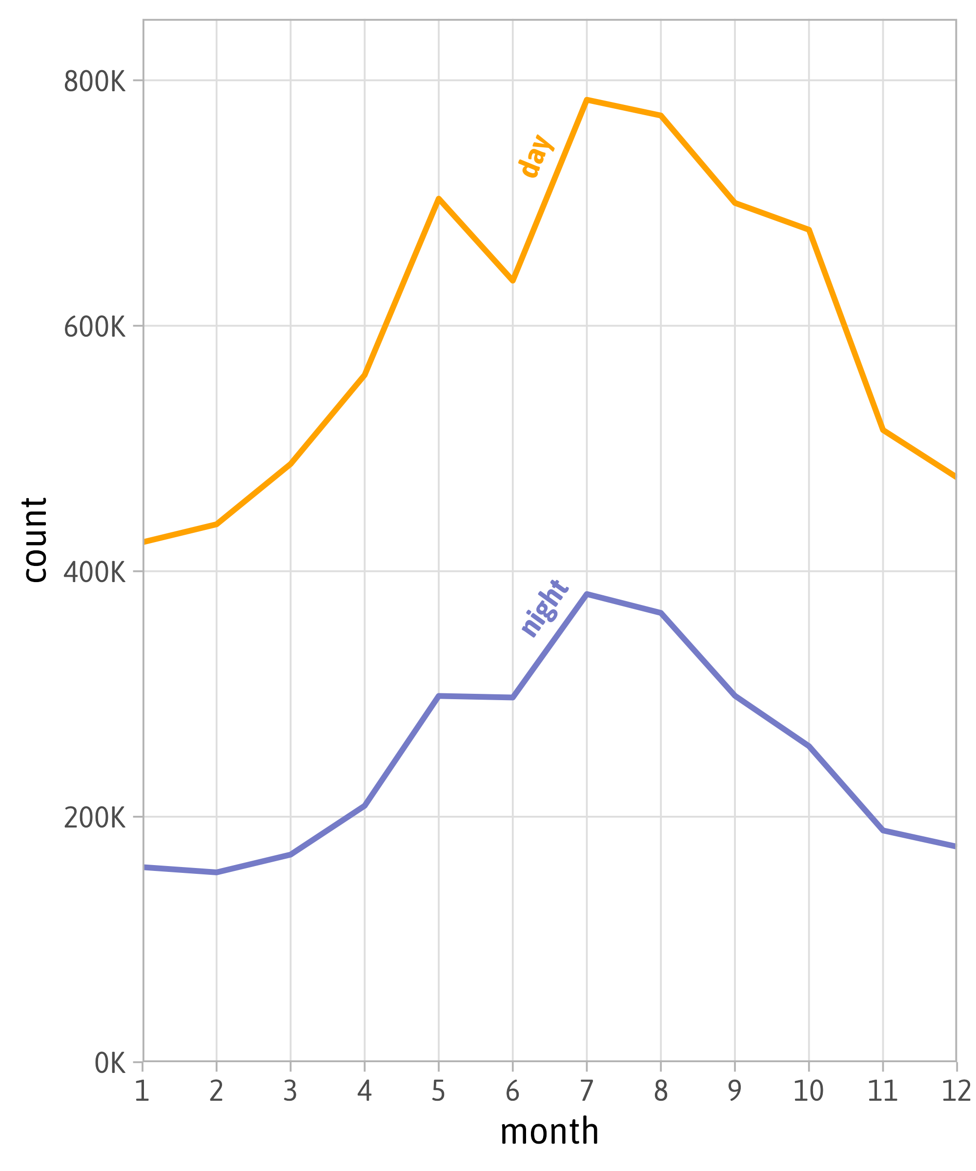
Annotations with {geomtextpath}
bikes |>
  filter(year == "2016") |>
  group_by(month, day_night) |>
  summarize(count = sum(count)) |>
  ggplot(aes(x = month, y = count,
             color = day_night,
             group = day_night)) +
  geomtextpath::geom_textline(
    aes(label = day_night),
    linewidth = 1,
    vjust = -.5,
    family = "Asap SemiCondensed",
    fontface = "bold"
  ) +
  coord_cartesian(expand = FALSE) +
  scale_y_continuous(
    labels = scales::label_comma(
      scale = 1/10^3, suffix = "K"
    ),
    limits = c(0, 850000)
  ) +
  scale_color_manual(
    values = c("#FFA200", "#757BC7"),
    guide = "none"
  )
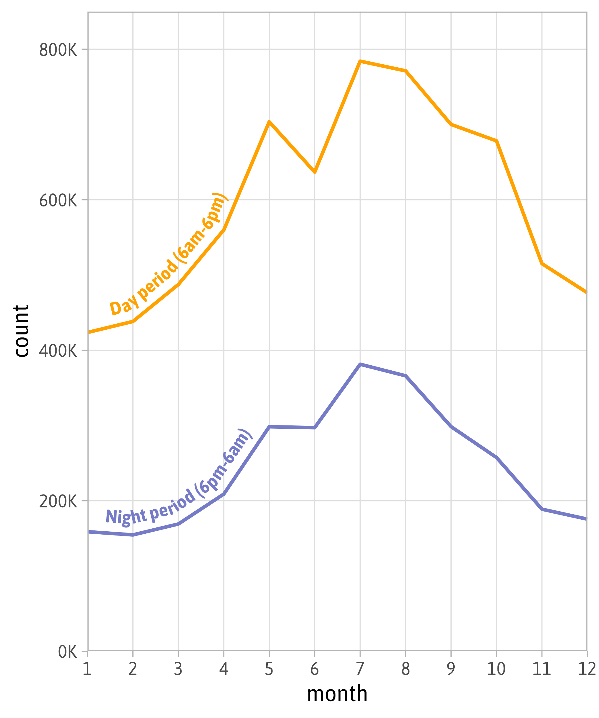
Annotations with {geomtextpath}
bikes |>
  filter(year == "2016") |>
  group_by(month, day_night) |>
  summarize(count = sum(count)) |>
  mutate(day_night = if_else(
    day_night == "day",
    "Day period (6am-6pm)",
    "Night period (6pm-6am)"
  )) |>
  ggplot(aes(x = month, y = count,
             color = day_night,
             group = day_night)) +
  geomtextpath::geom_textline(
    aes(label = day_night),
    linewidth = 1,
    vjust = -.5,
    hjust = .05,
    family = "Asap SemiCondensed",
    fontface = "bold"
  ) +
  coord_cartesian(expand = FALSE) +
  scale_y_continuous(
    labels = scales::label_comma(
      scale = 1/10^3, suffix = "K"
    ),
    limits = c(0, 850000)
  ) +
  scale_color_manual(
    values = c("#FFA200", "#757BC7"),
    guide = "none"
  )
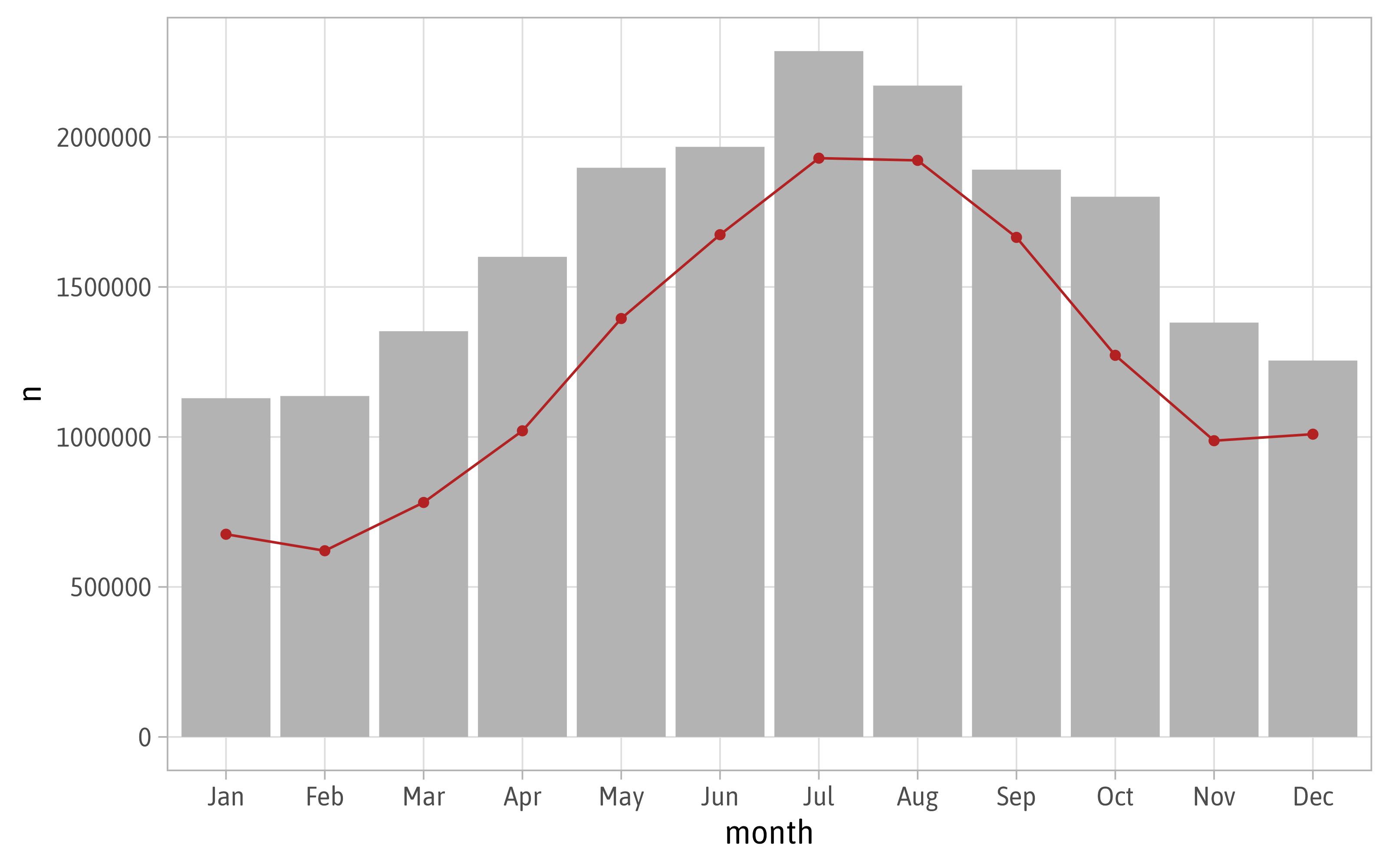
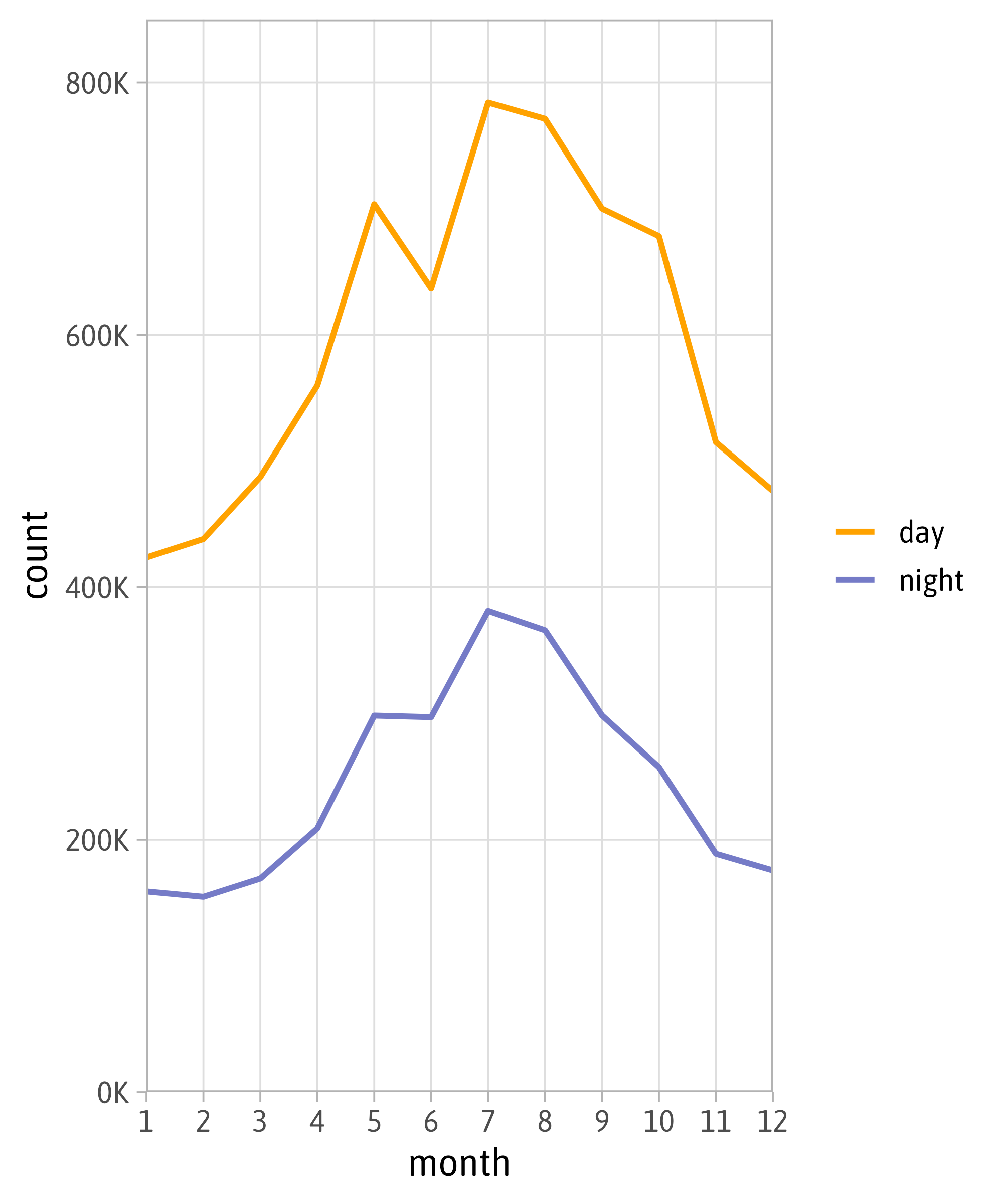
Line Chart with stat_summary()
bikes |>
  filter(year == "2016") |>
  ggplot(aes(x = month, y = count,
             color = day_night,
             group = day_night)) +
  stat_summary(
    geom = "line", fun = sum,
    linewidth = 1
  ) +
  coord_cartesian(expand = FALSE) +
  scale_y_continuous(
    labels = scales::label_comma(
      scale = 1/10^3, suffix = "K"
    ),
    limits = c(0, 850000)
  ) +
  scale_color_manual(
    values = c("#FFA200", "#757BC7"),
    name = NULL
  )
Line Chart with stat_summary()
bikes |>
  filter(year == "2016") |>
  ggplot(aes(x = month, y = count,
             color = day_night,
             group = day_night)) +
  geomtextpath::geom_textline(
    aes(label = day_night),
    stat = "summary", fun = sum,
    linewidth = 1
  ) +
  coord_cartesian(expand = FALSE) +
  scale_y_continuous(
    labels = scales::label_comma(
      scale = 1/10^3, suffix = "K"
    ),
    limits = c(0, 850000)
  ) +
  scale_color_manual(
    values = c("#FFA200", "#757BC7"),
    name = NULL
  )
# A tibble: 142 × 6
   country     continent  year lifeExp       pop gdpPercap
   <fct>       <fct>     <int>   <dbl>     <int>     <dbl>
 1 Afghanistan Asia       2007    43.8  31889923      975.
 2 Albania     Europe     2007    76.4   3600523     5937.
 3 Algeria     Africa     2007    72.3  33333216     6223.
 4 Angola      Africa     2007    42.7  12420476     4797.
 5 Argentina   Americas   2007    75.3  40301927    12779.
 6 Australia   Oceania    2007    81.2  20434176    34435.
 7 Austria     Europe     2007    79.8   8199783    36126.
 8 Bahrain     Asia       2007    75.6    708573    29796.
 9 Bangladesh  Asia       2007    64.1 150448339     1391.
10 Belgium     Europe     2007    79.4  10392226    33693.
# ℹ 132 more rows