library(ggplot2)
library(dplyr)

bikes <- readr::read_csv(
  here::here("data", "london-bikes-custom.csv"),
  col_types = "Dcfffilllddddc"
)

theme_set(theme_light(base_size = 14, base_family = "Asap SemiCondensed"))

theme_update(
  panel.grid.minor = element_blank(),
  plot.title = element_text(face = "bold"),
  plot.title.position = "plot"
)Engaging and Beautiful Data Visualizations with ggplot2
Working with Colors
Default Color Palettes: Categorical
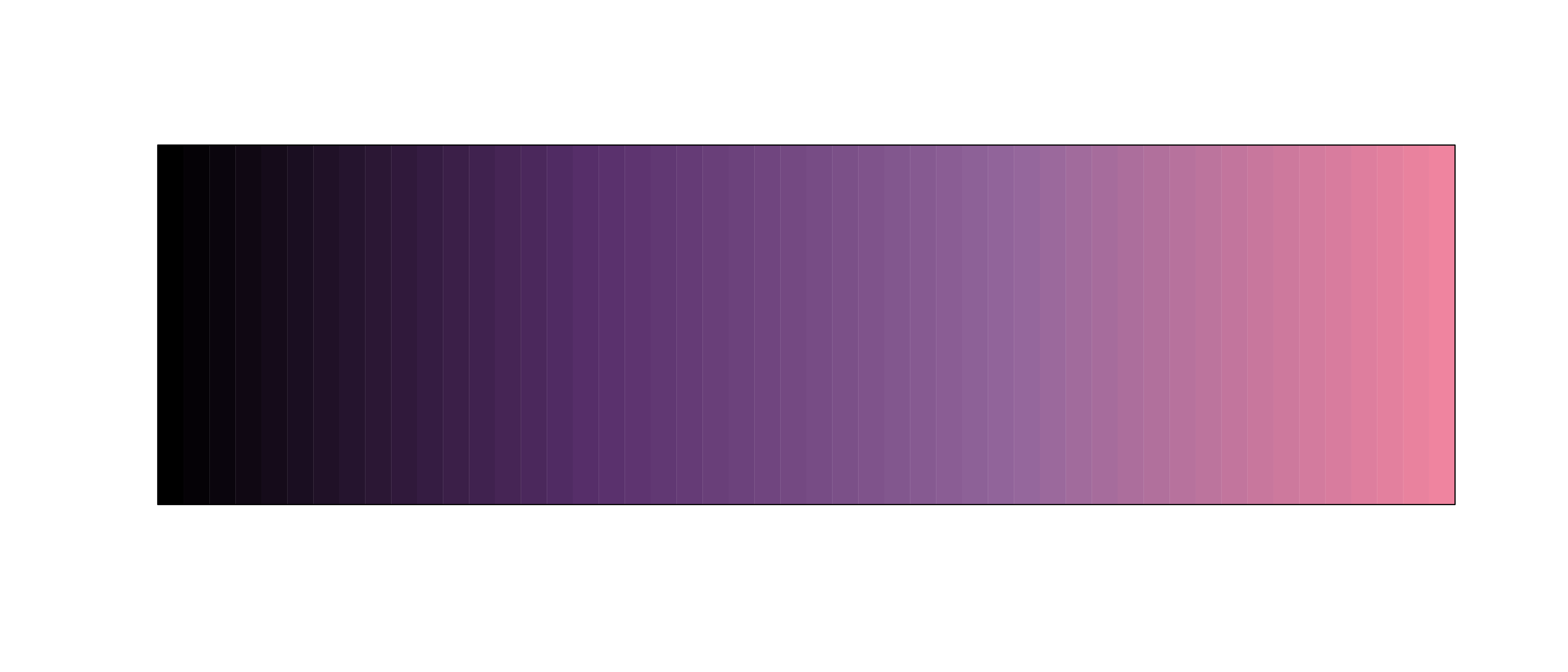
Default Color Palettes: Sequential

The Viridis Color Palettes
![Figure 1 in Nuñez, Anderton & Renslow (2018) PLoS One: Example of a misleading colormap. Comparison between different colormaps overlaid onto the test image by Kovesi and a nanoscale secondary ion mass spectrometry image. Colormaps are as follows: (a) perceptually uniform grayscale, (b) jet, (c) jet as it appears to someone with red-green colorblindness, and (d) viridis [1], the current gold standard colormap. Below each NanoSIMS image is a corresponding “colormap-data perceptual sensitivity” (CDPS) plot, which compares perceptual differences of the colormap to actual, underlying data differences. m is the slope of the fitted line and r2 is the coefficient of determination calculated using a simple linear regression. An example of how the data may be misinterpreted are evident in the bright yellow spots in (b) and (c), which appear to represent significantly higher values than the surrounding regions. However, in fact, the dark red (in b) and dark yellow (in c) actually represent the highest values. For someone who is red-green colorblind, this is made even more difficult to interpret due to the broad, bright band in the center of the colormap with values that are difficult to distinguish.](img/viridis-performance.png)
Nuñez, Anderton & Renslow (2018), PloS One 13:e0199239. DOI: 10.1371/journal.pone.0199239
The Viridis Color Palettes
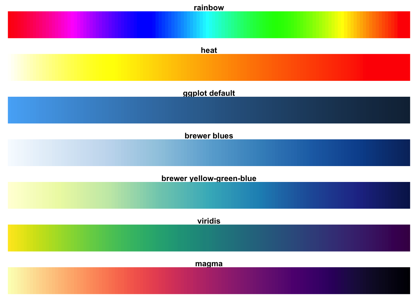
Palette comparison of commonly used sequential color palettes in R from the {viridis} vignette
The Viridis Color Palettes
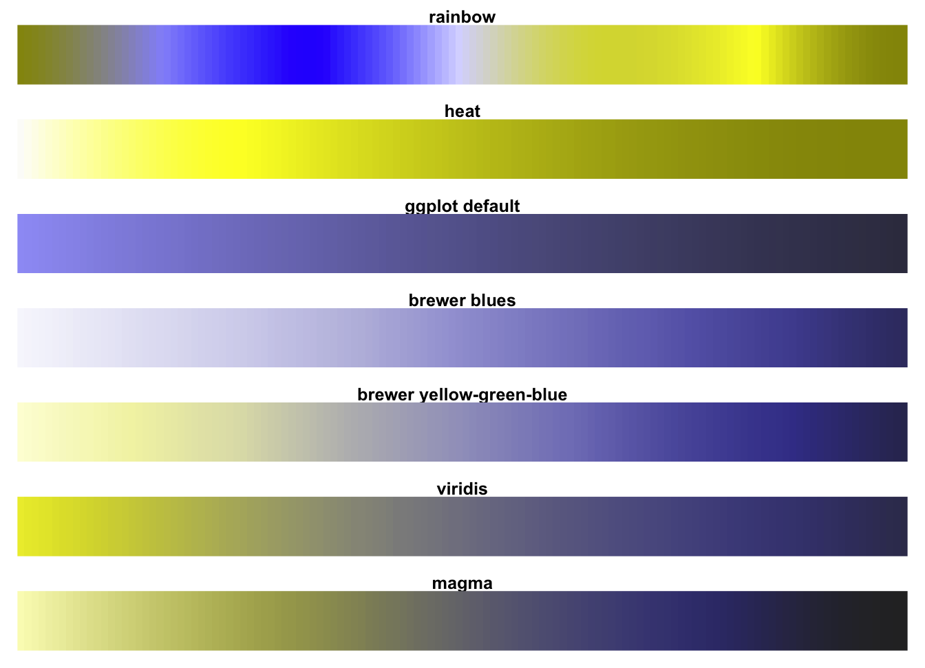
Palette comparison, as seen by a person with Deuteranopia, from the {viridis} vignette
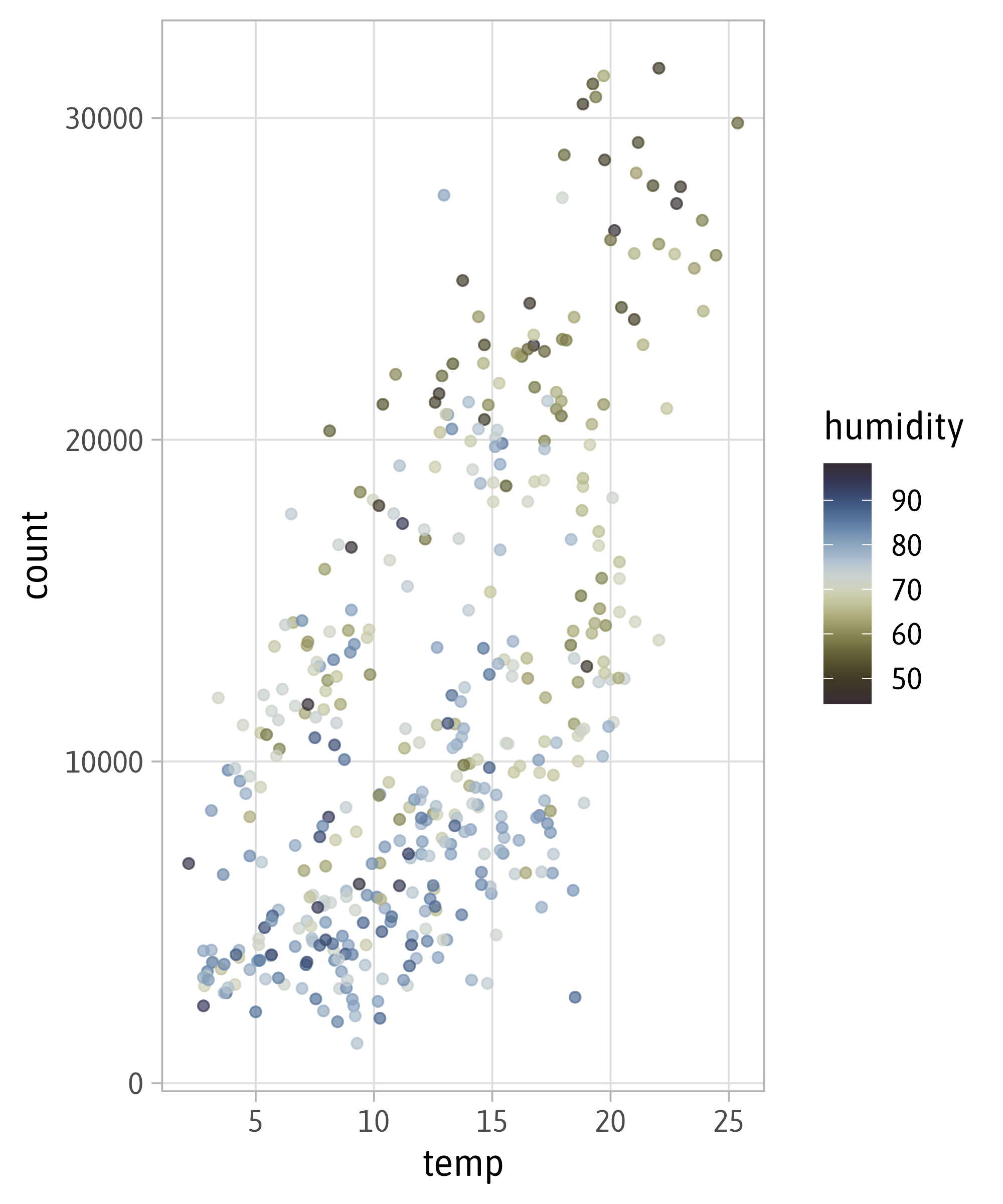
Pre-Defined Color Palettes: Viridis
Pre-Defined Color Palettes: Viridis
Pre-Defined Color Palettes: Viridis
Pre-Defined Color Palettes: Viridis
Pre-Defined Color Palettes: Viridis
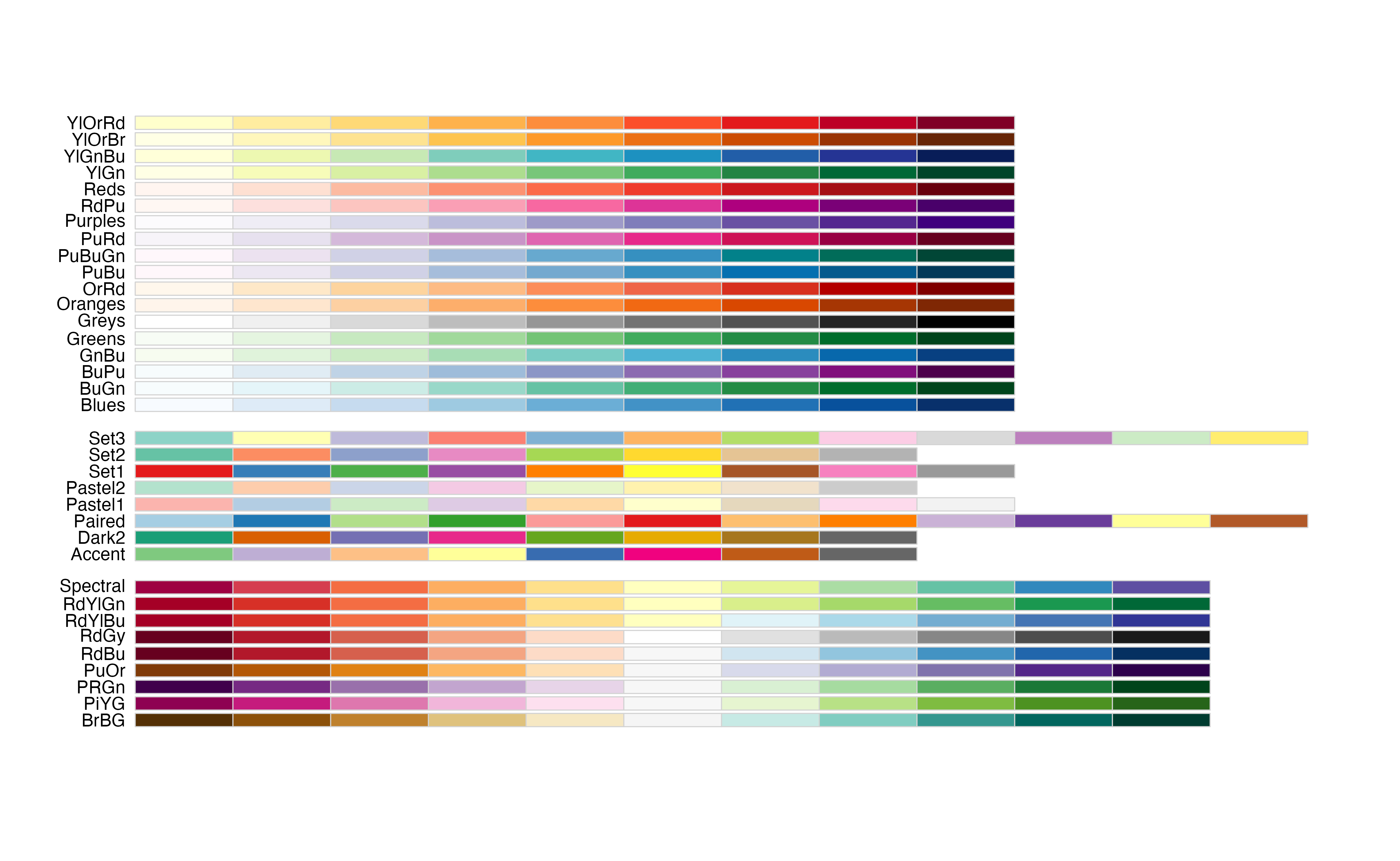
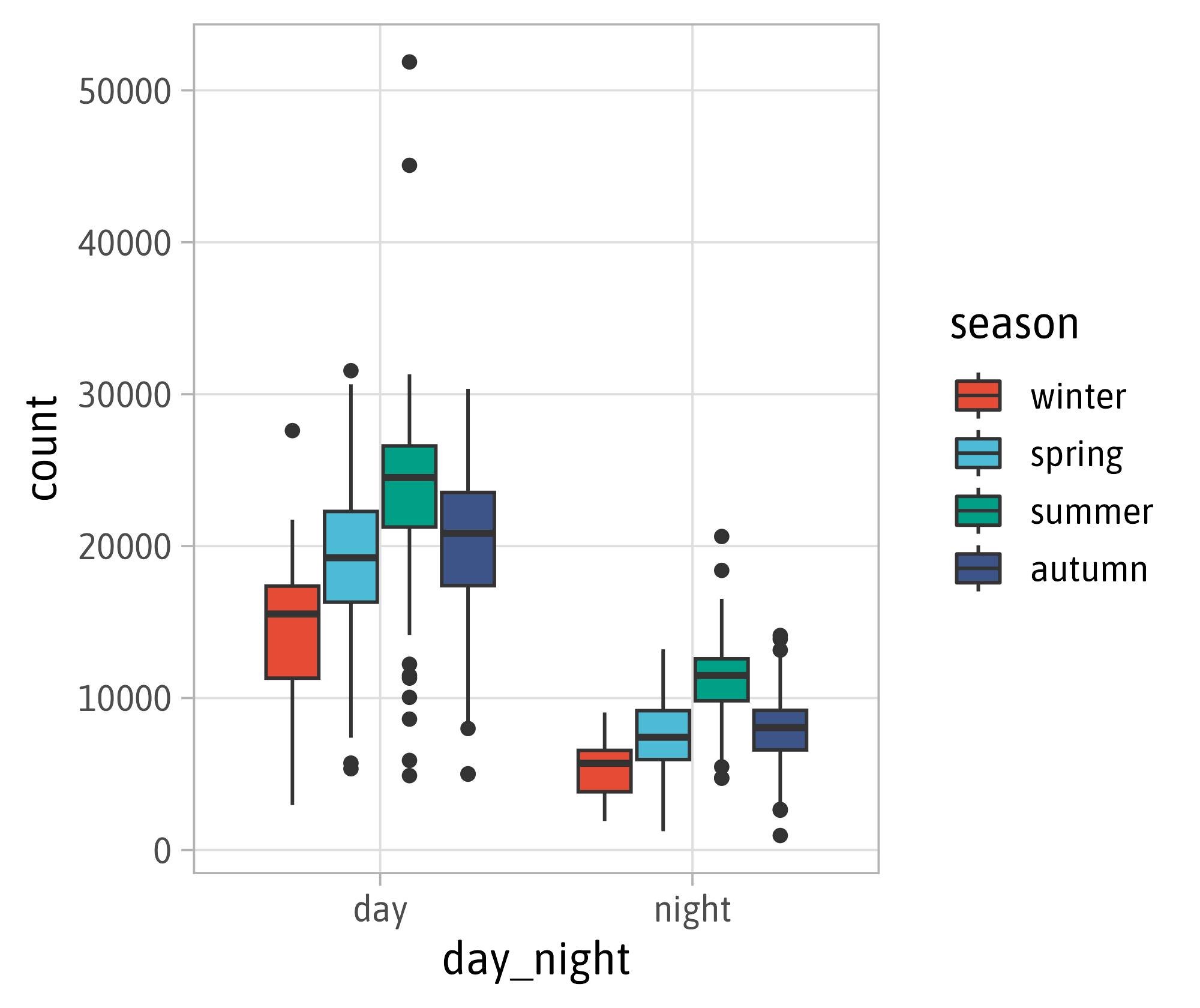
Pre-Defined Color Palettes: ColorBrewer
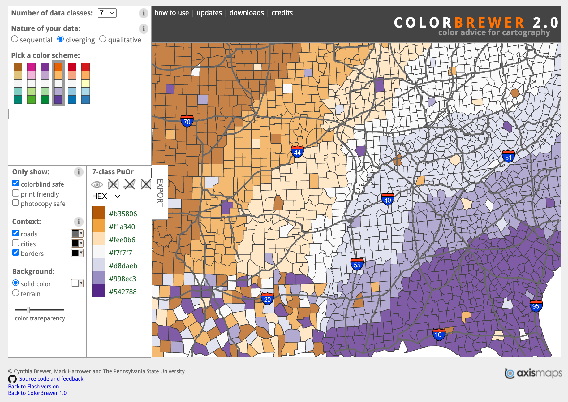
The ColorBrewer project: colorbrewer2.org
Pre-Defined Color Palettes: ColorBrewer
Pre-Defined Color Palettes: ColorBrewer
Pre-Defined Color Palettes: ColorBrewer
Pre-Defined Color Palettes: ColorBrewer

Pre-Defined Color Palettes: ColorBrewer
Pre-Defined Color Palettes: ColorBrewer
{rcartocolor}

{rcartocolor}
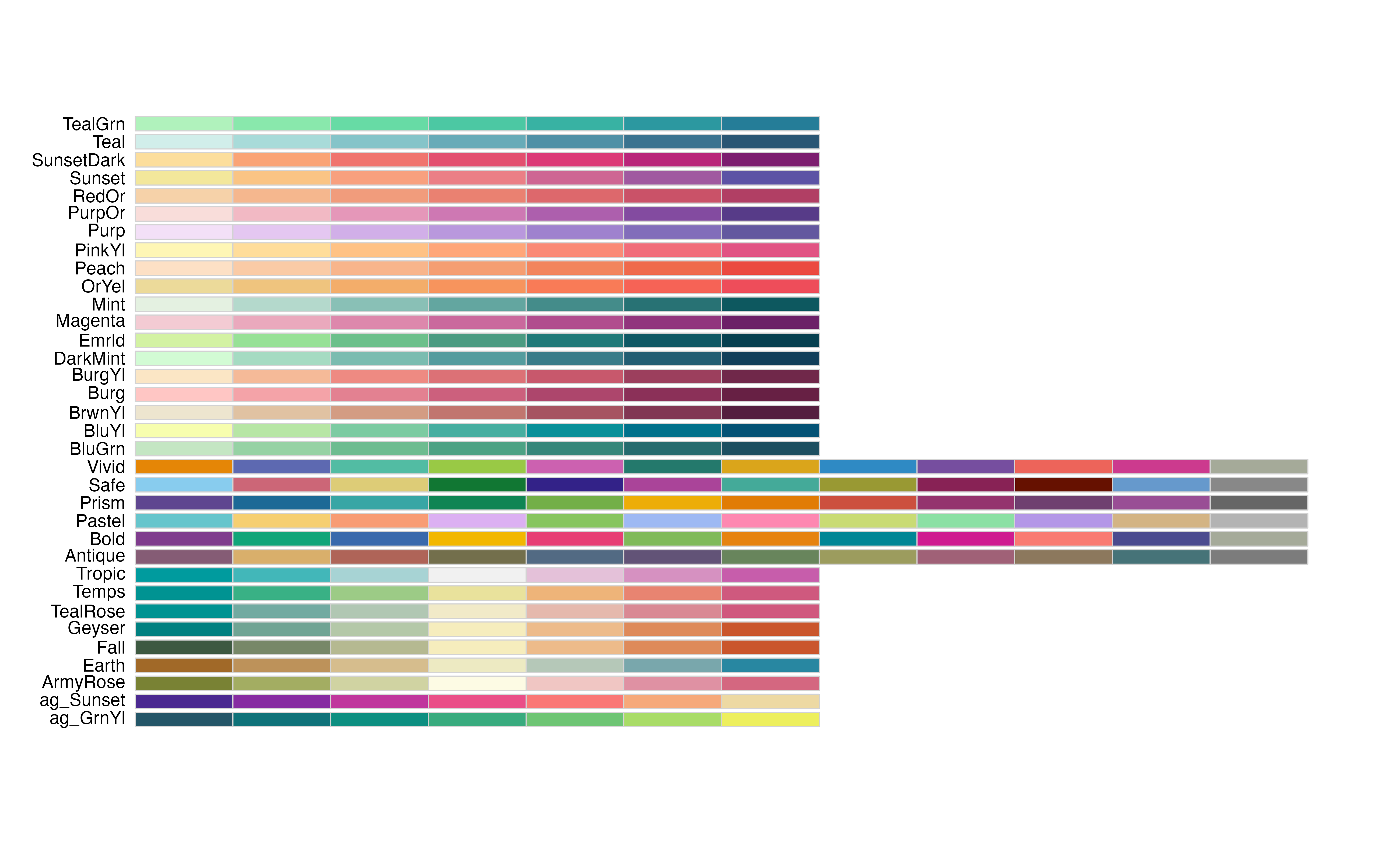
{rcartocolor}
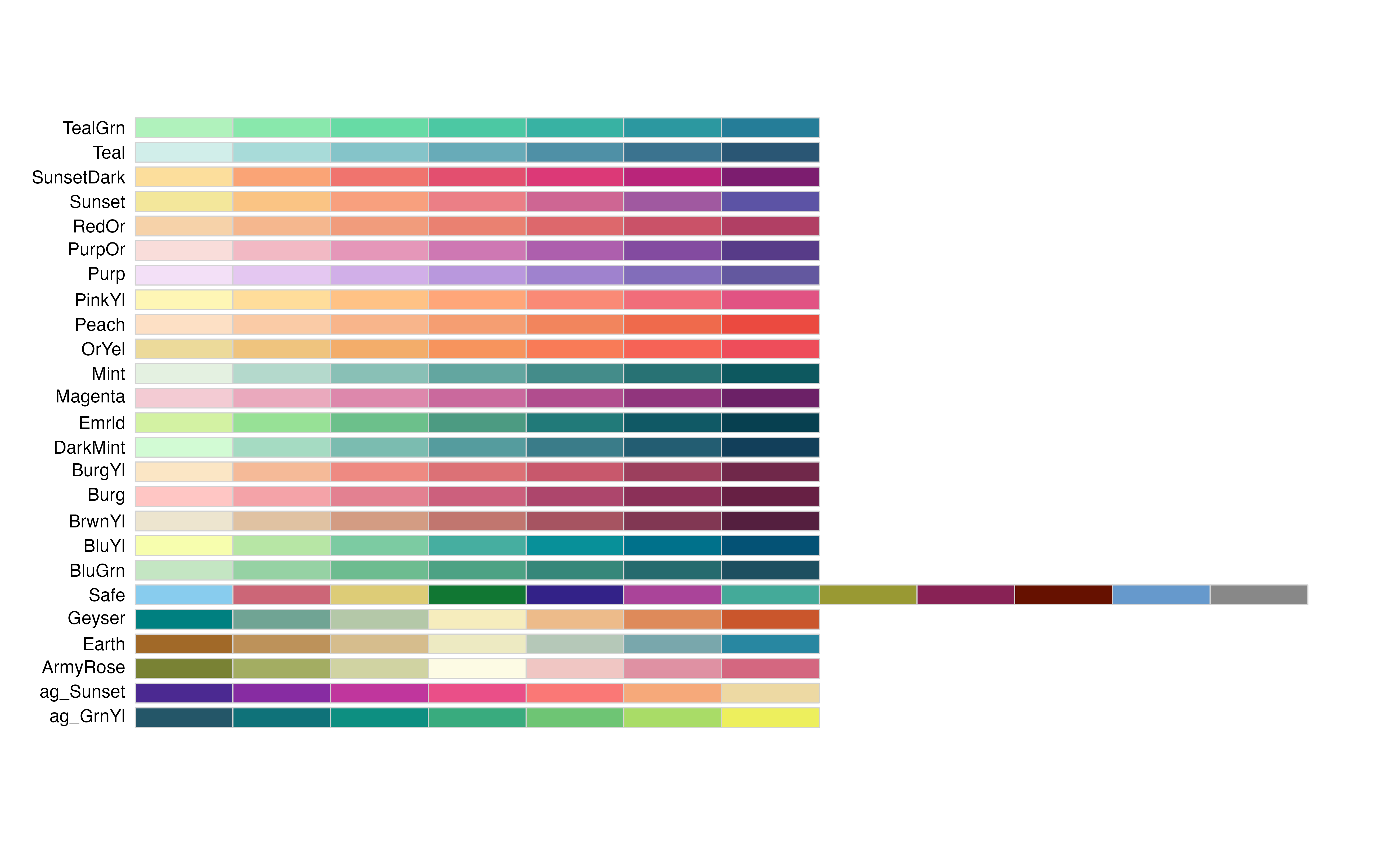
{rcartocolor}
{scico}
{scico}
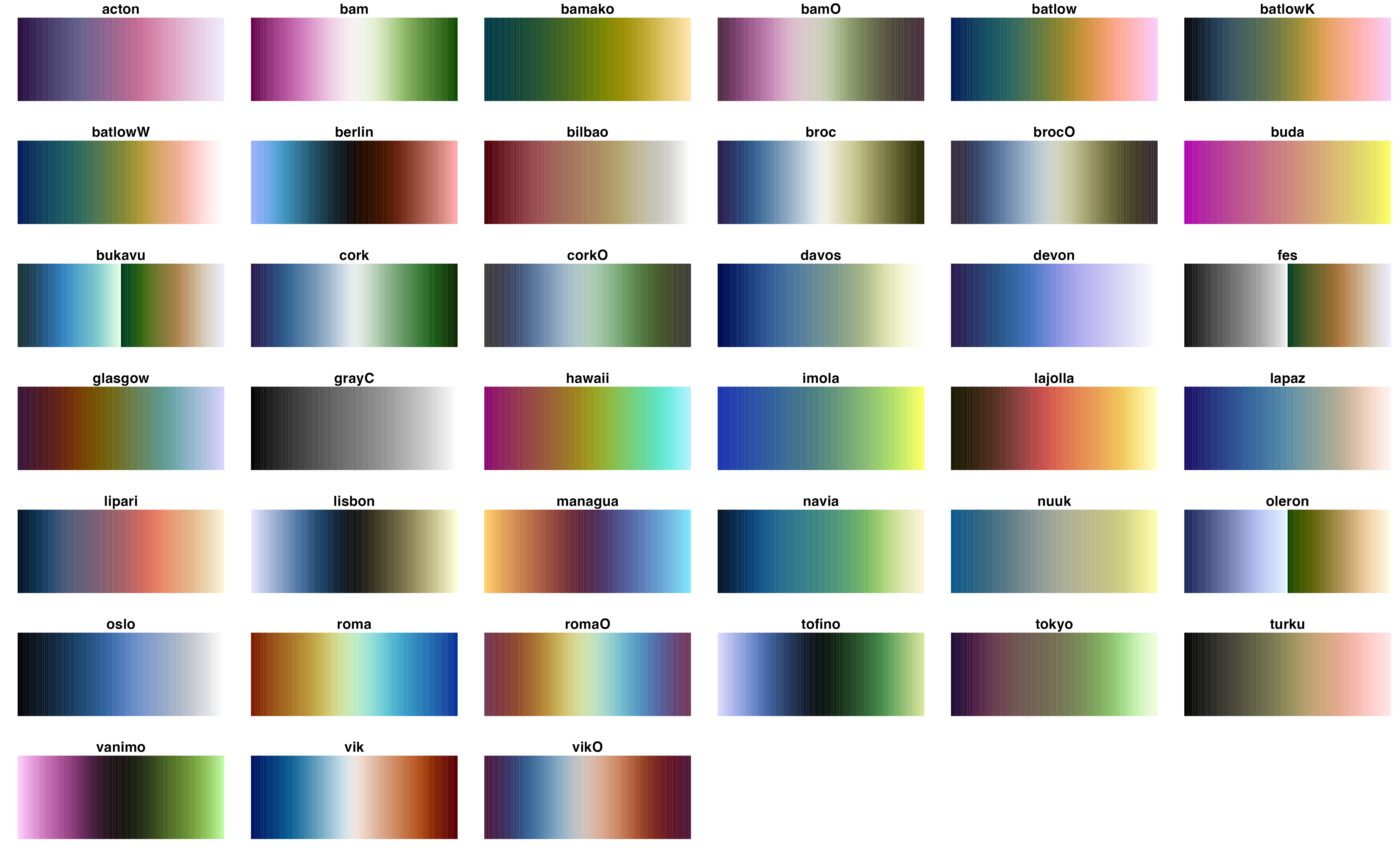
{scico}
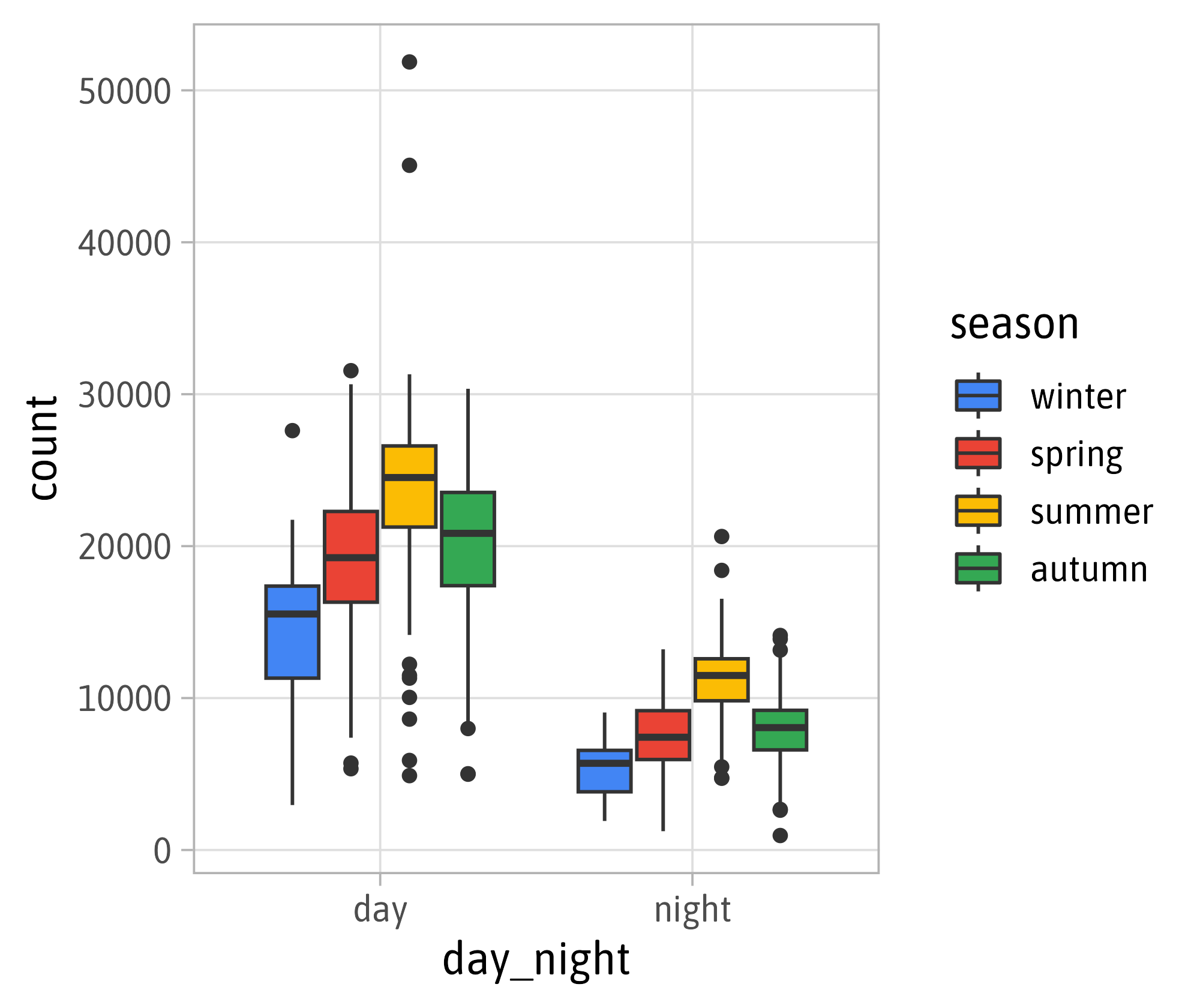
{ggsci} and {ggthemes}
{MetBrewer}
{MetBrewer}
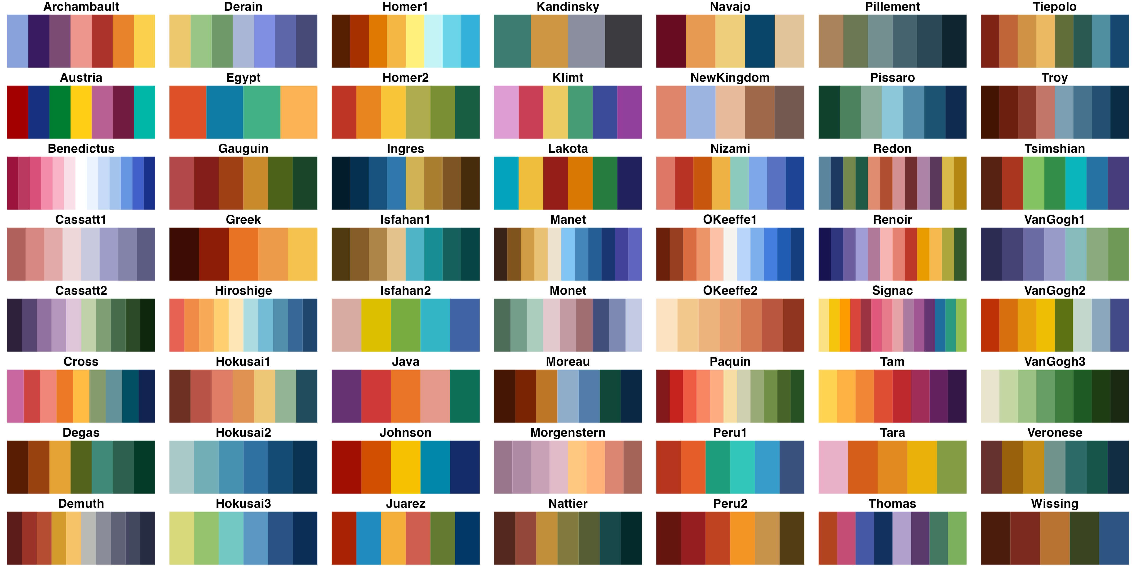
{MetBrewer}
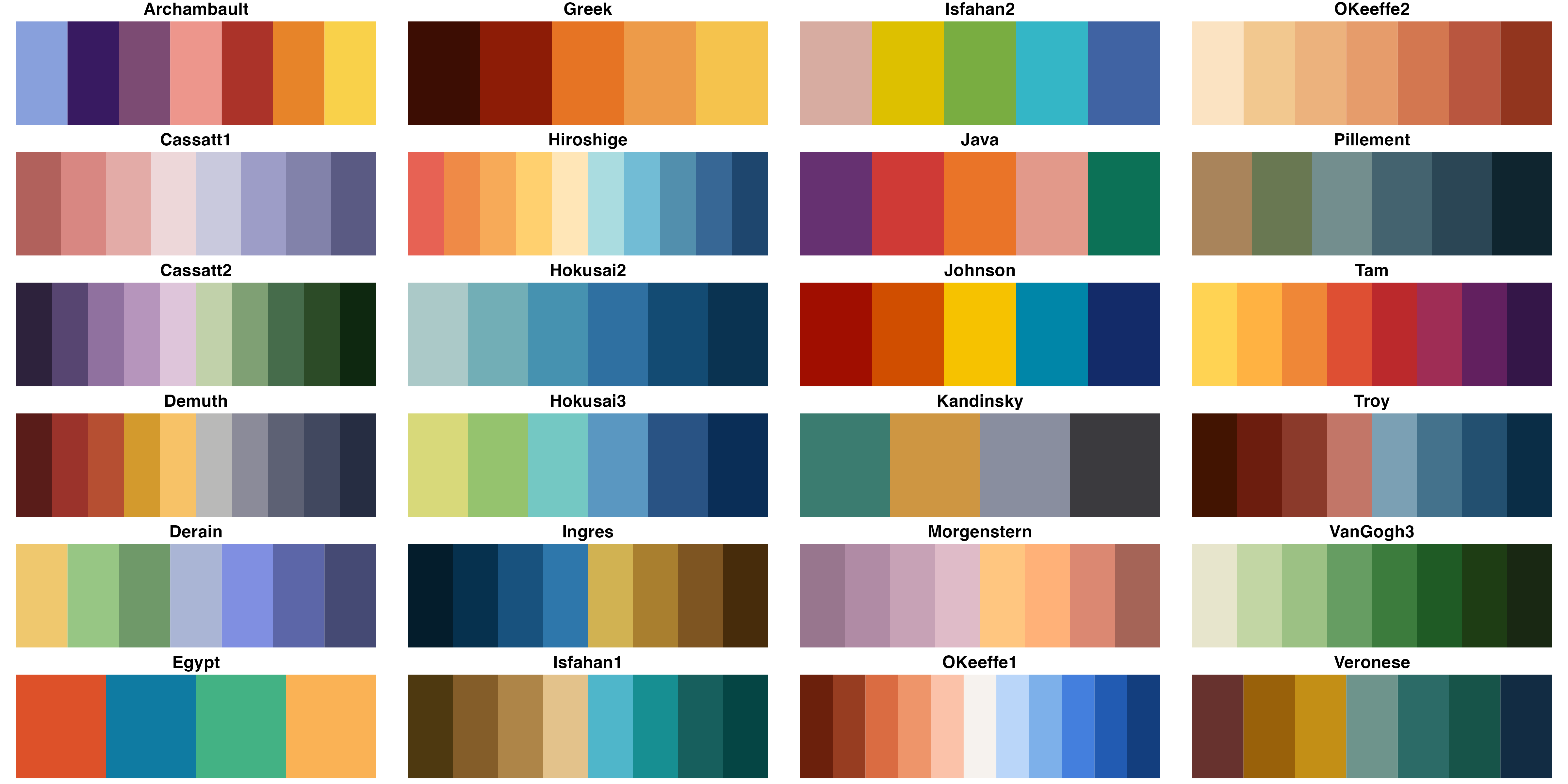
{MetBrewer}
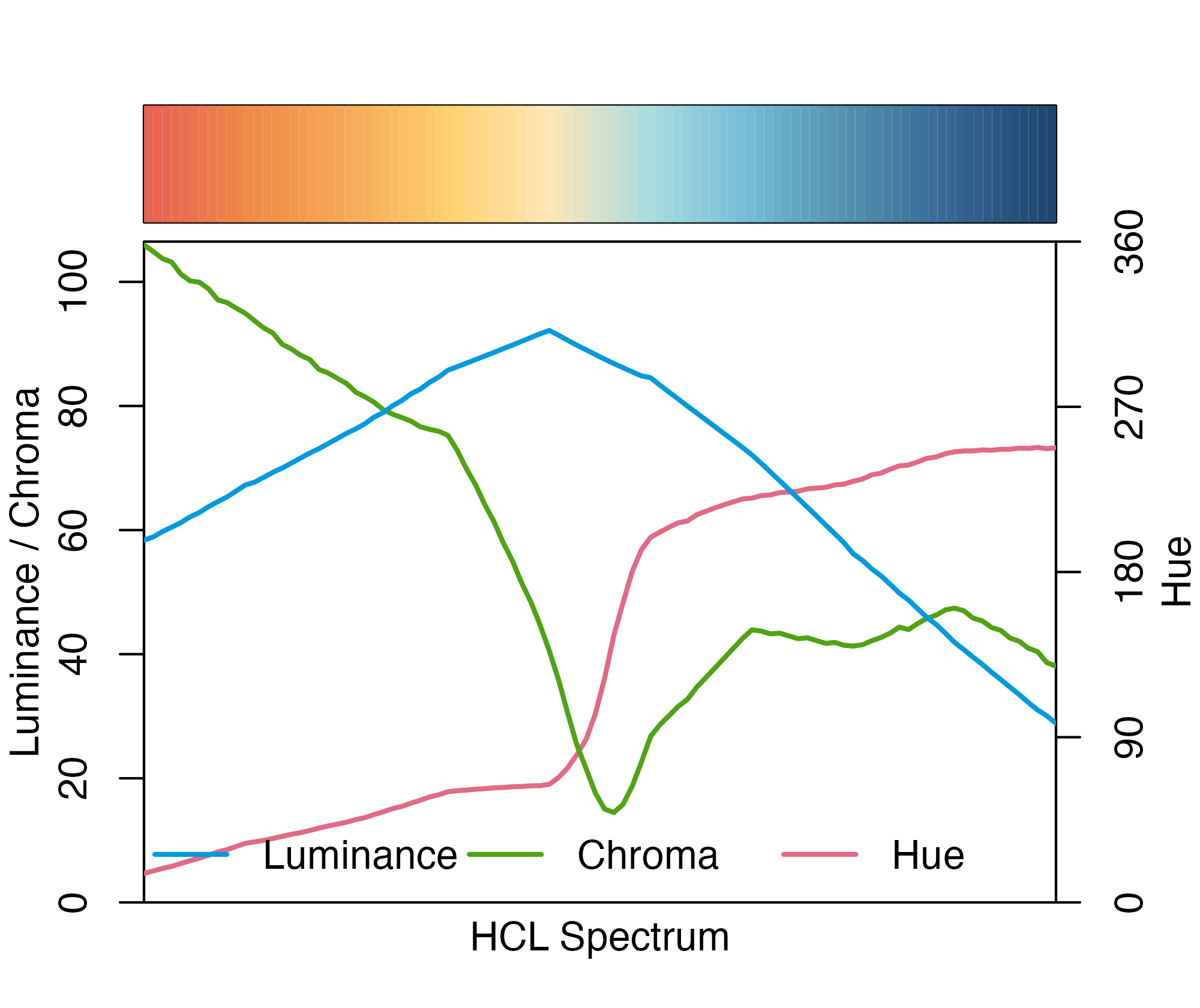
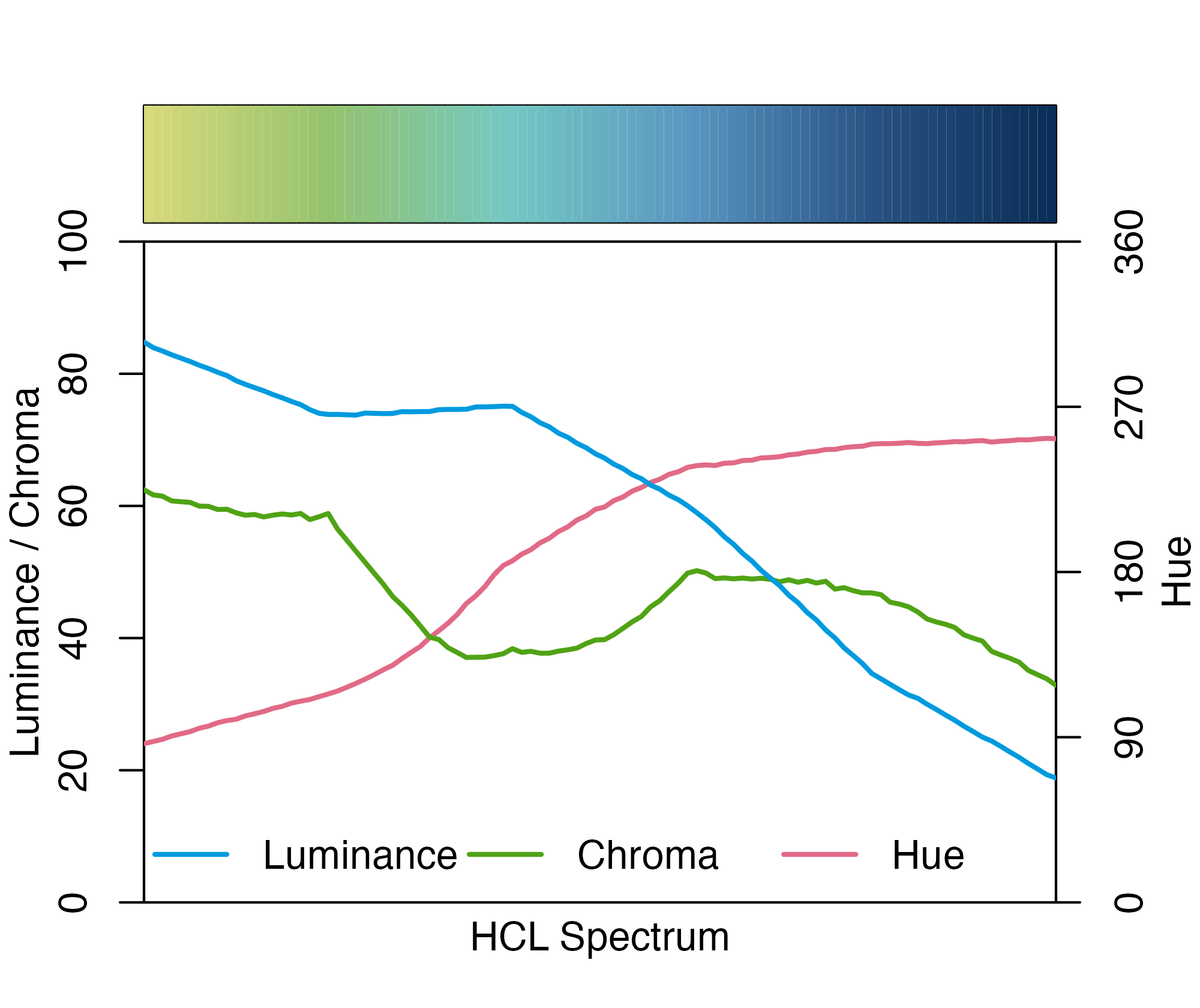
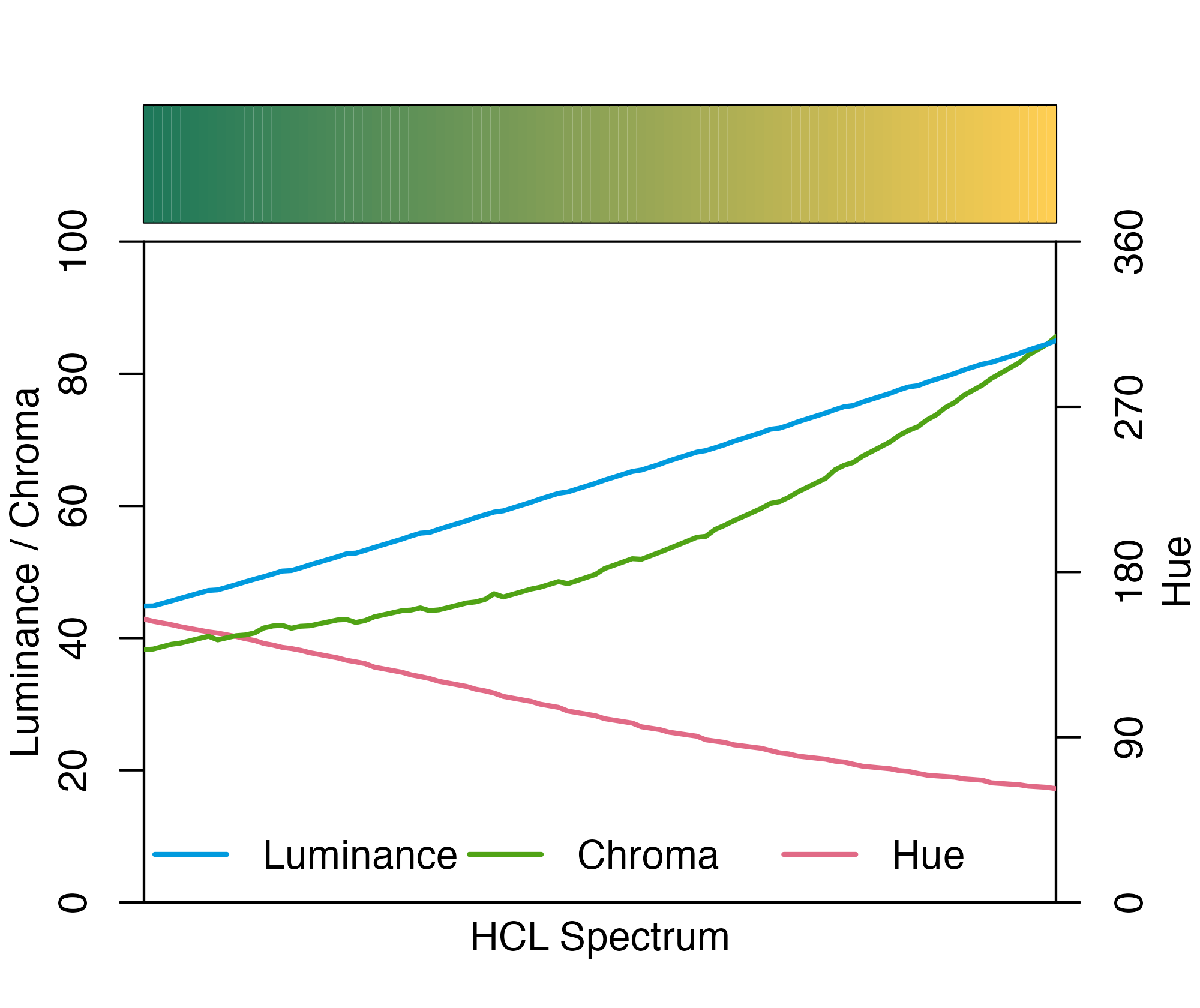
Evaluate HCL Spectrum
More on how to evaluate color palettes: HCLwizard and colorspace.
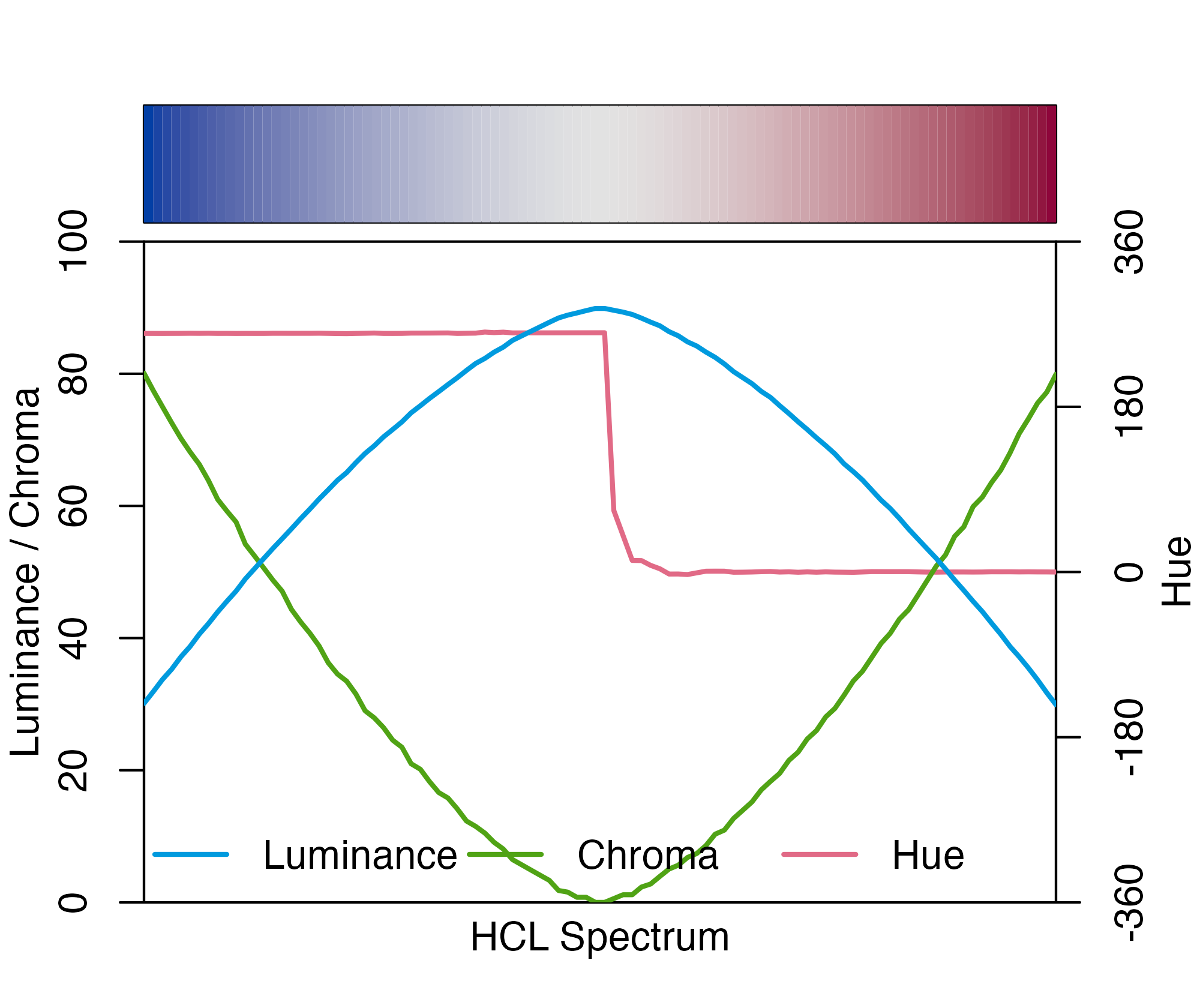
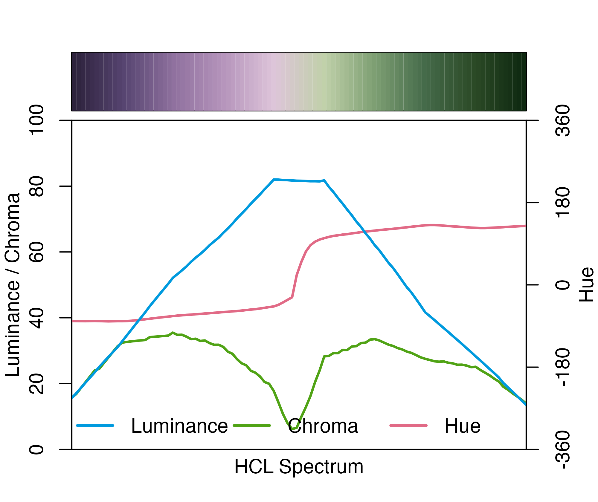
Evaluate HCL Spectrum
More on how to evaluate color palettes: HCLwizard and colorspace.
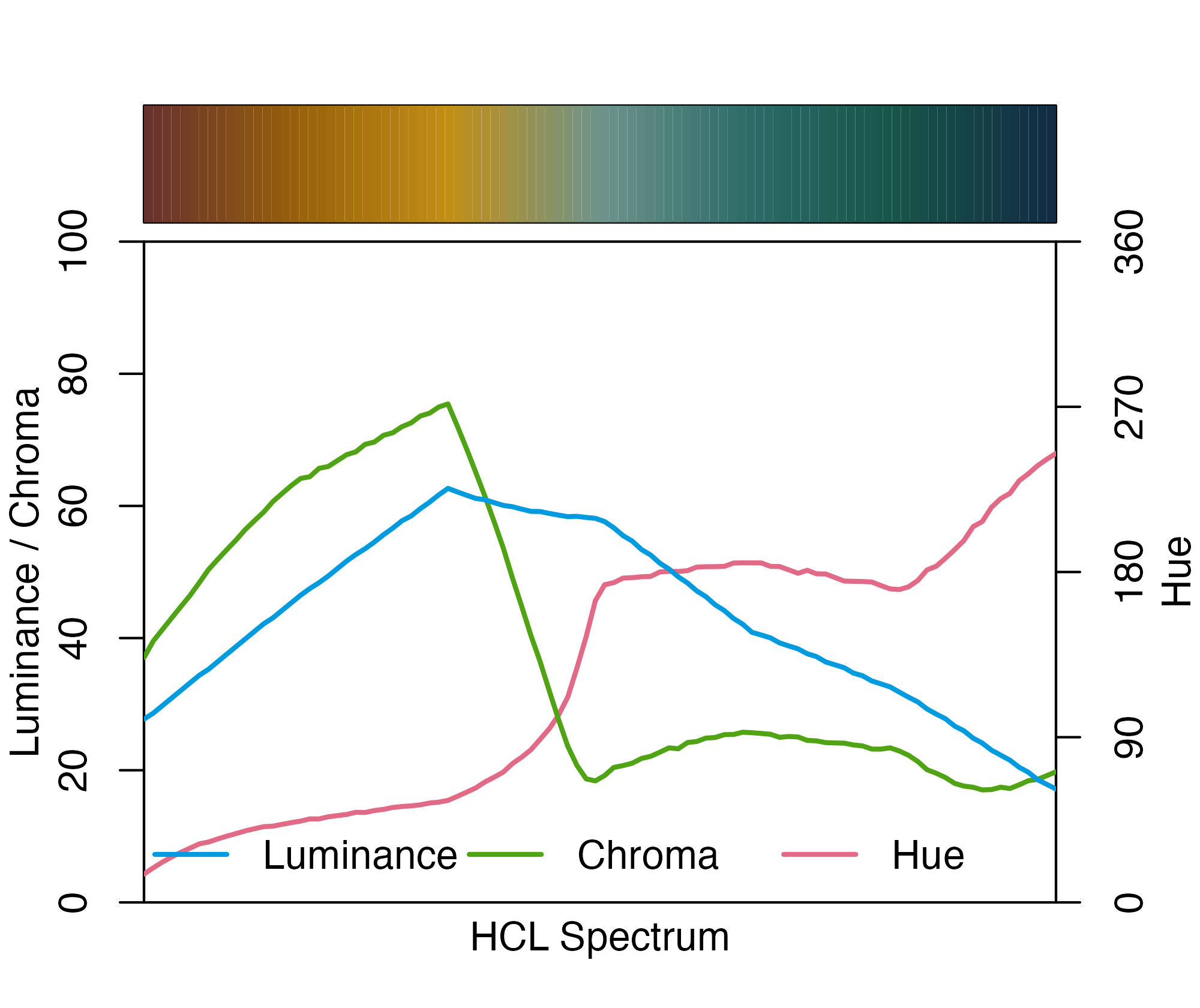
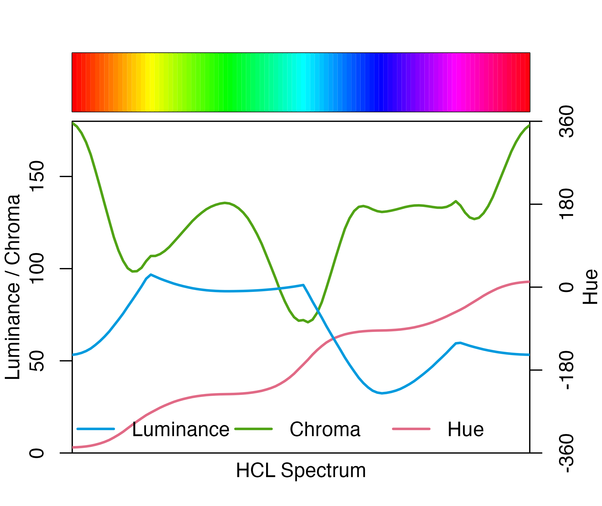
Evaluate HCL Spectrum
More on how to evaluate color palettes: HCLwizard and colorspace.
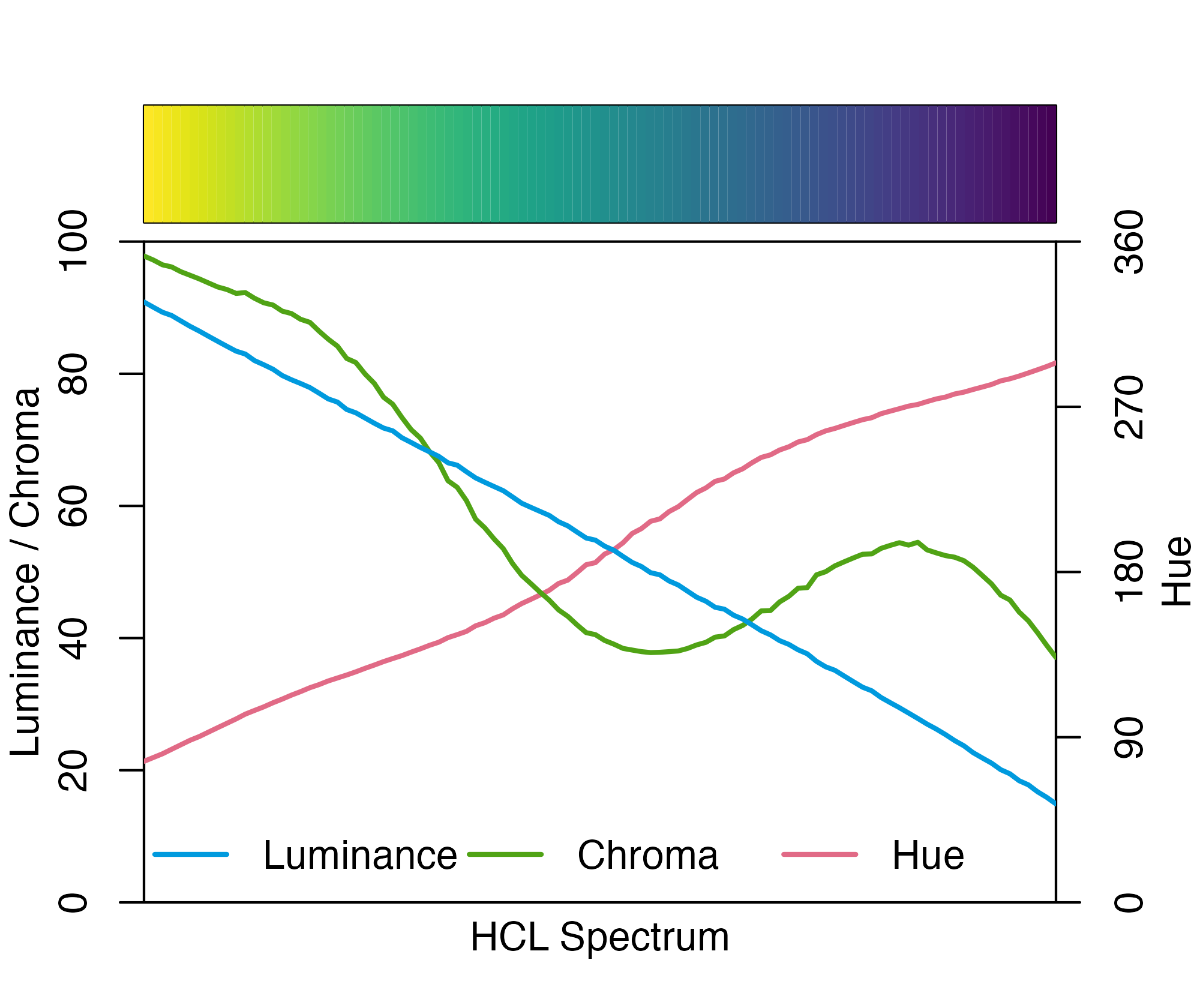
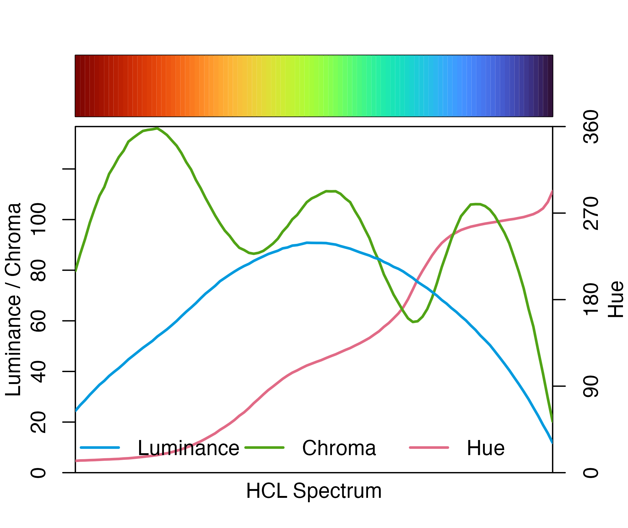
Evaluate HCL Spectrum
More on how to evaluate color palettes: HCLwizard and colorspace.
Customize Existing Palettes

Customize Existing Palettes
Customize Existing Palettes
Customize Existing Palettes

Customize Existing Palettes
Customize Existing Palettes

Customize Existing Palettes

Customize Existing Palettes
Customize Existing Palettes

Customize Existing Palettes
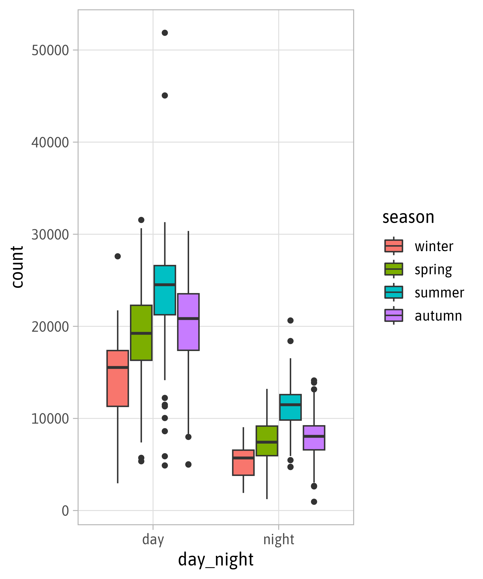
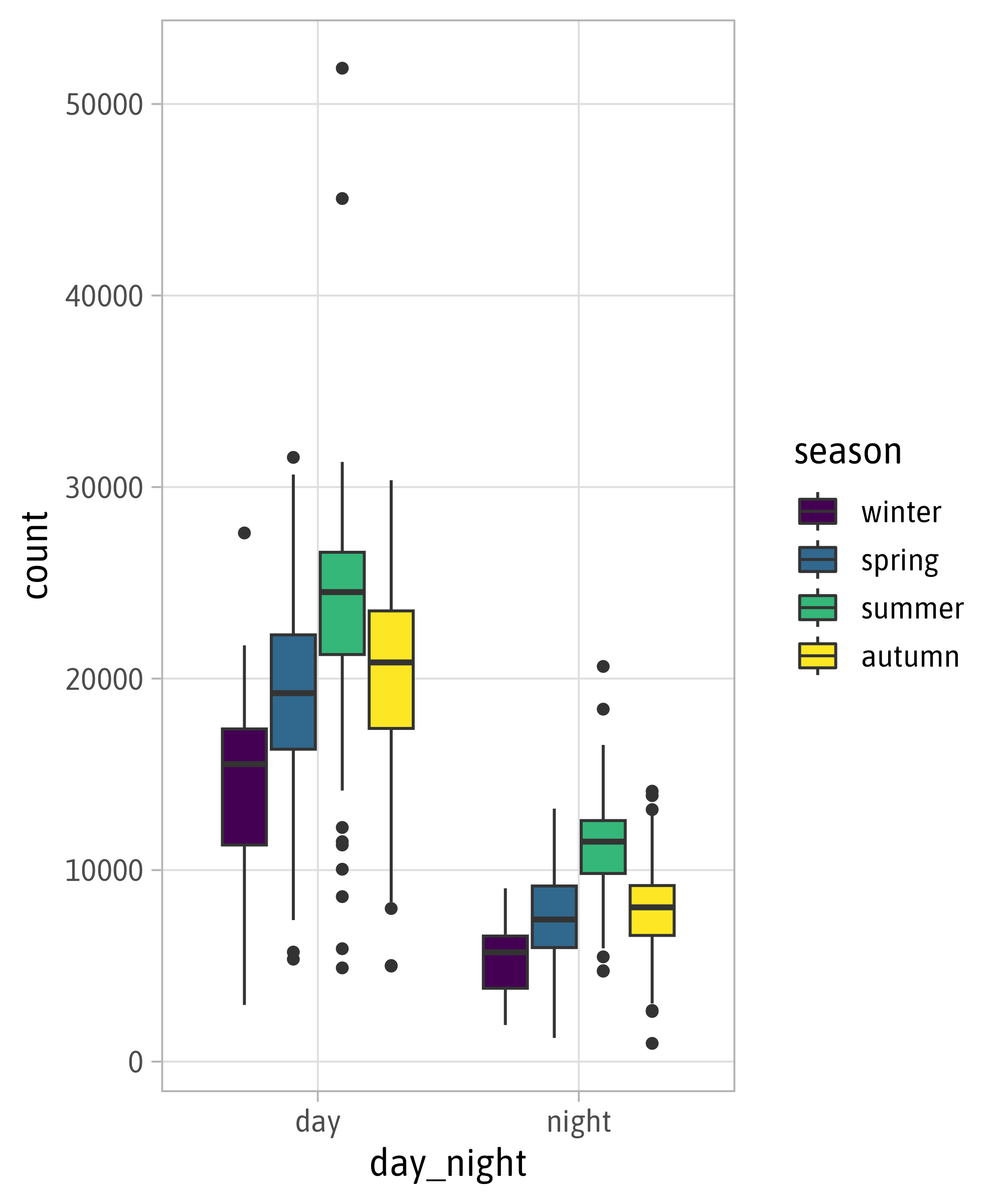
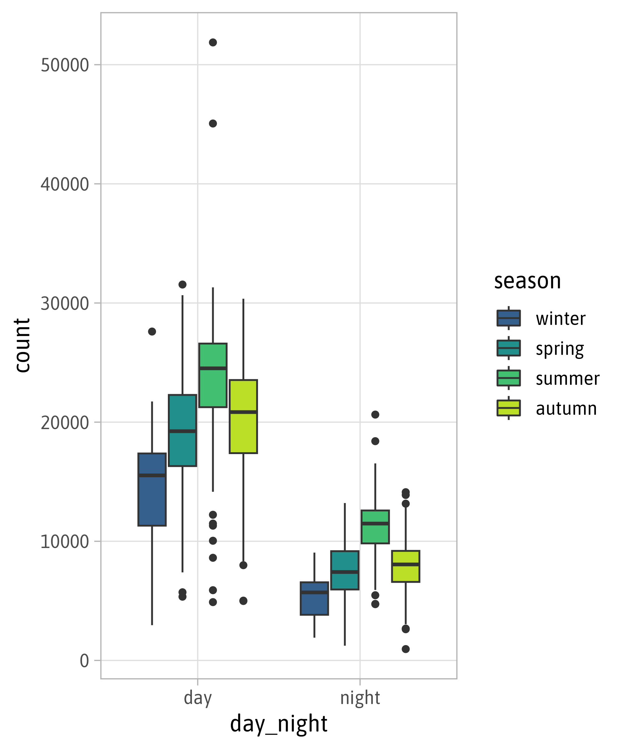
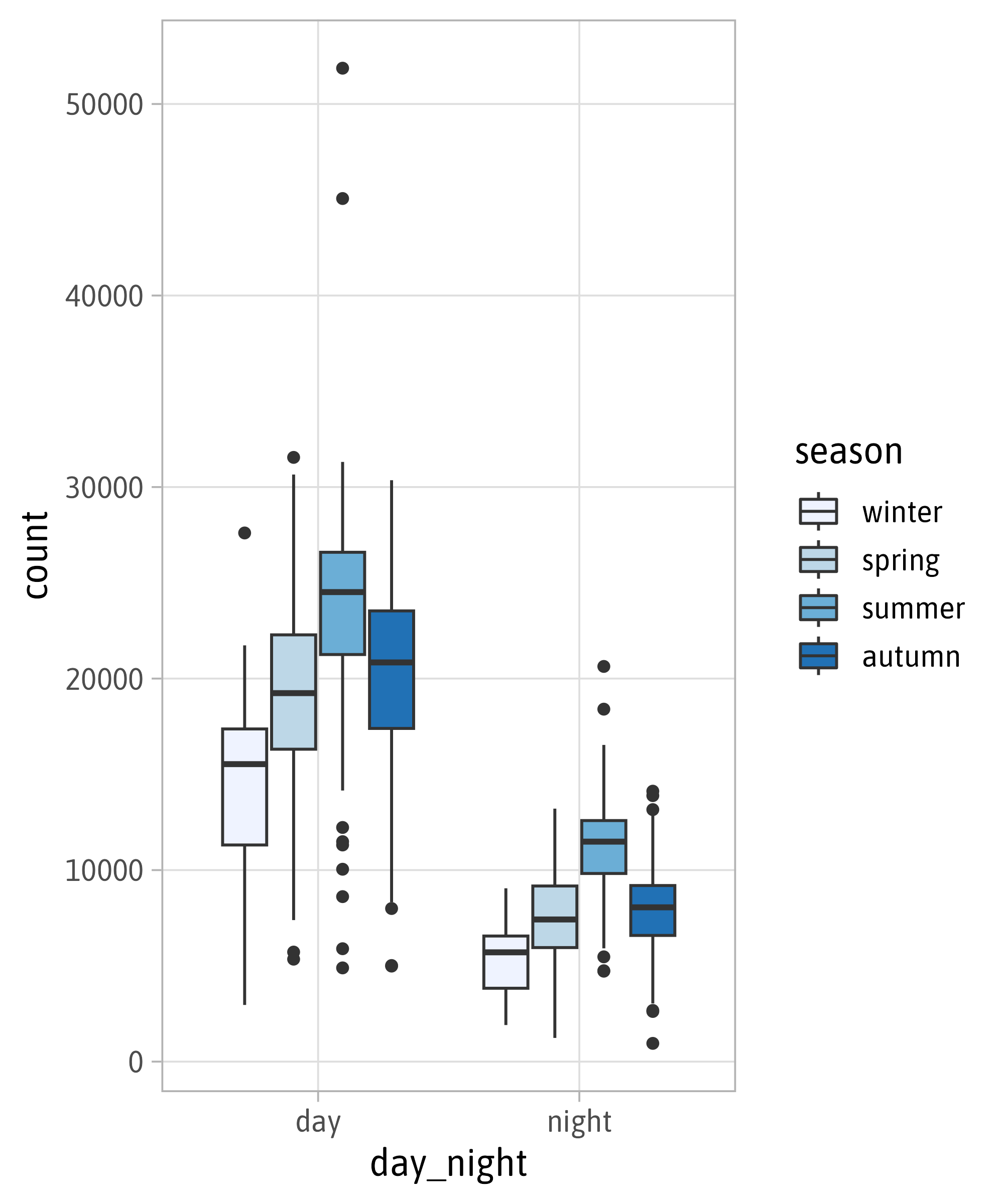
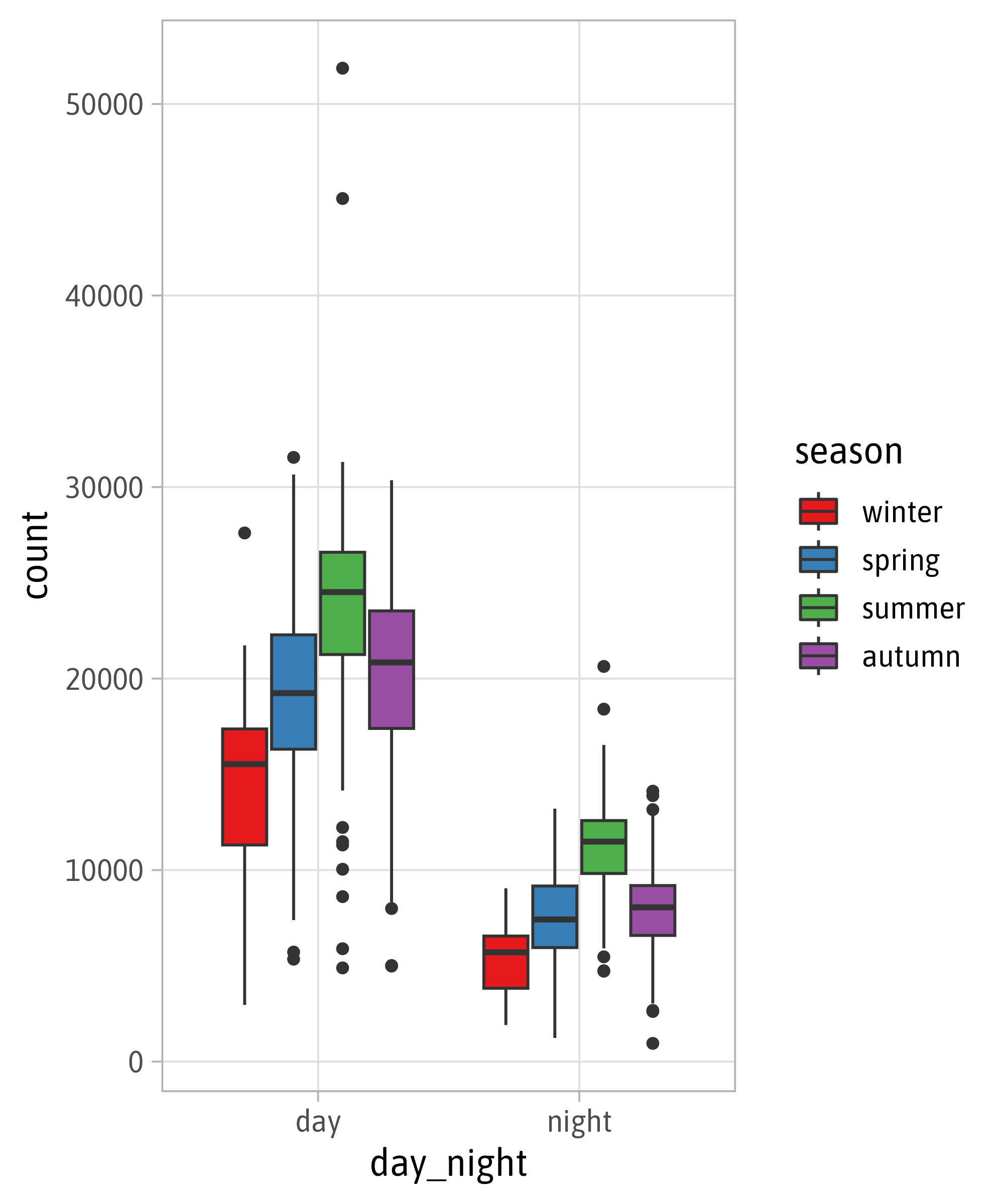
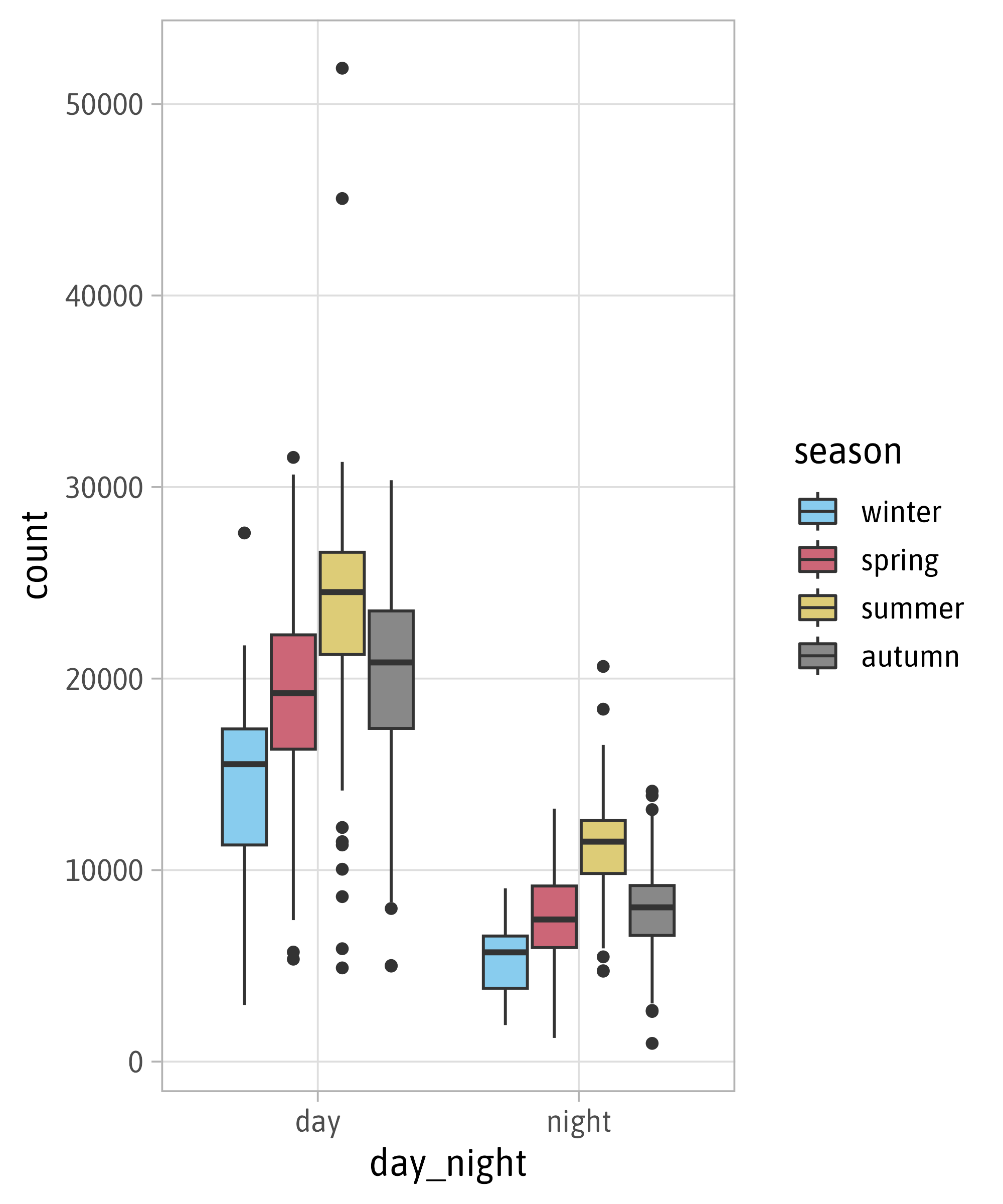
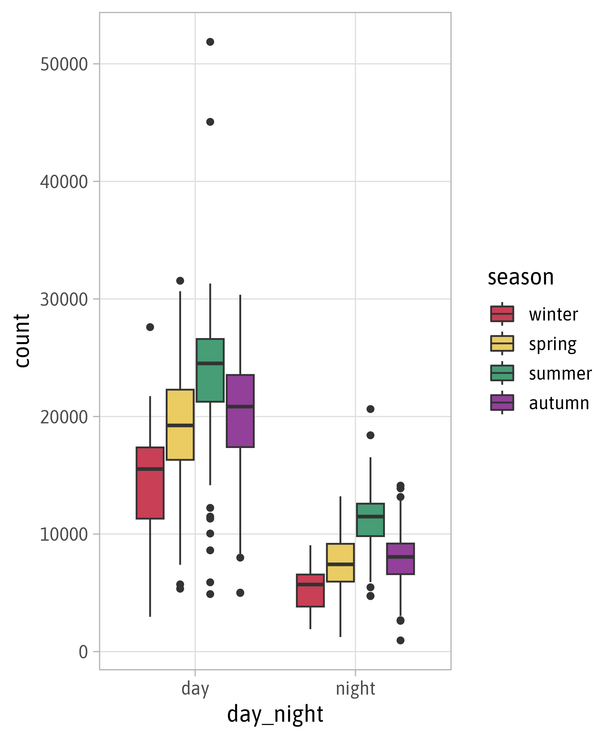
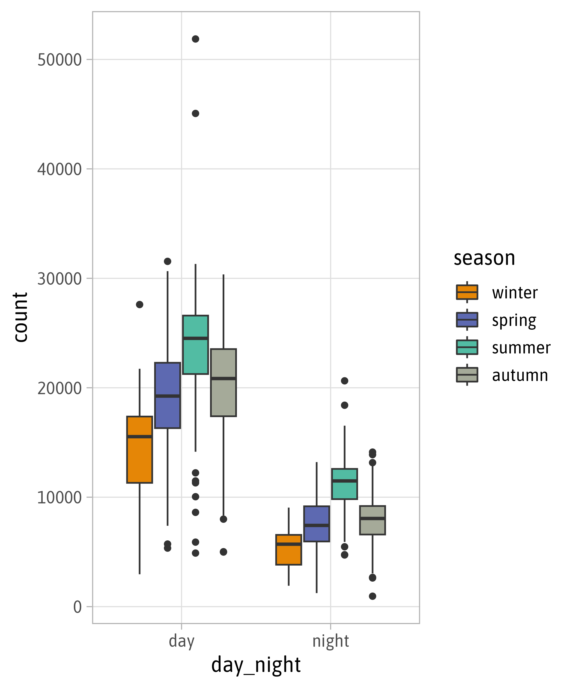
ggplot(bikes,
       aes(x = day_night, y = count)) +
  geom_boxplot(
    aes(color = season,
        fill = after_scale(
          clr_lighten(color, .7)
    )),
    outlier.shape = NA
  ) +
  geom_jitter(
    aes(color = season,
        color = after_scale(
          clr_darken(color, .4)
    )),
    position = position_jitterdodge(
      dodge.width = .75,
      jitter.width = .2
    ),
    alpha = .3, size = .6
  ) +
  scale_color_manual(
    values = carto_custom
  ) +
  theme(legend.position = "top")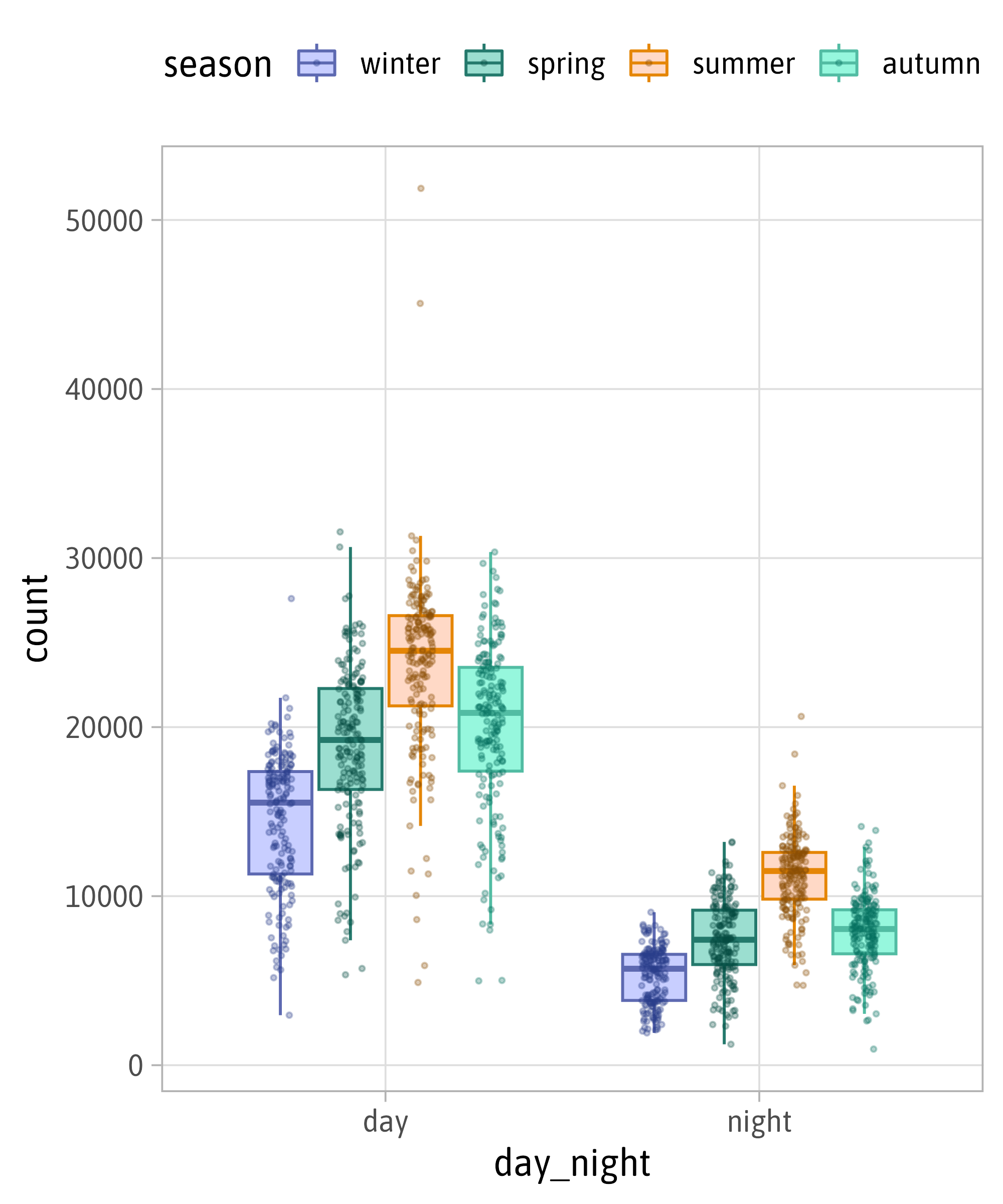
Create Sequential Palettes
Create Diverging Palettes
Create Diverging Palettes

Create Diverging Palettes
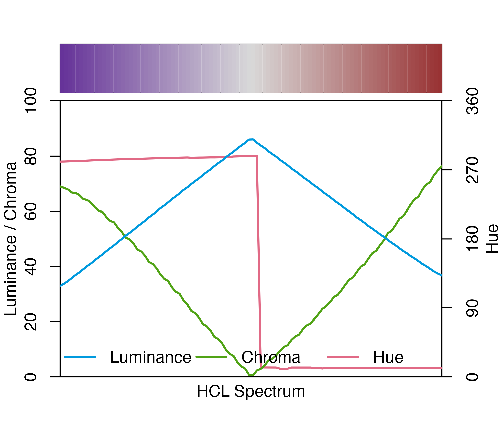
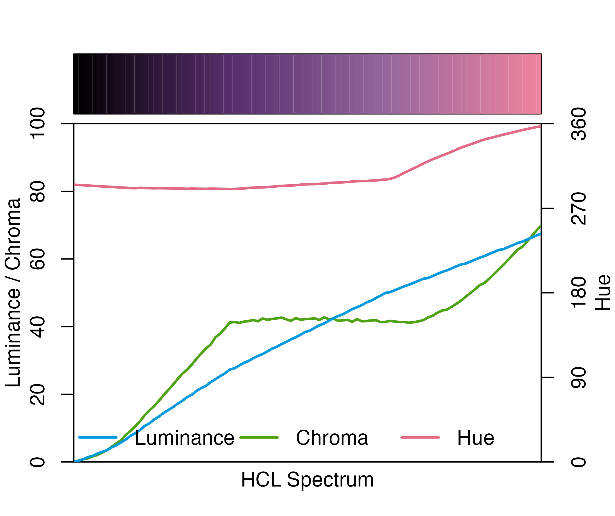
Evaluate HCL Spectrum
More on how to evaluate color palettes: HCLwizard and colorspace.
Create Any Palette

Create Any Palette
Create Any Palette
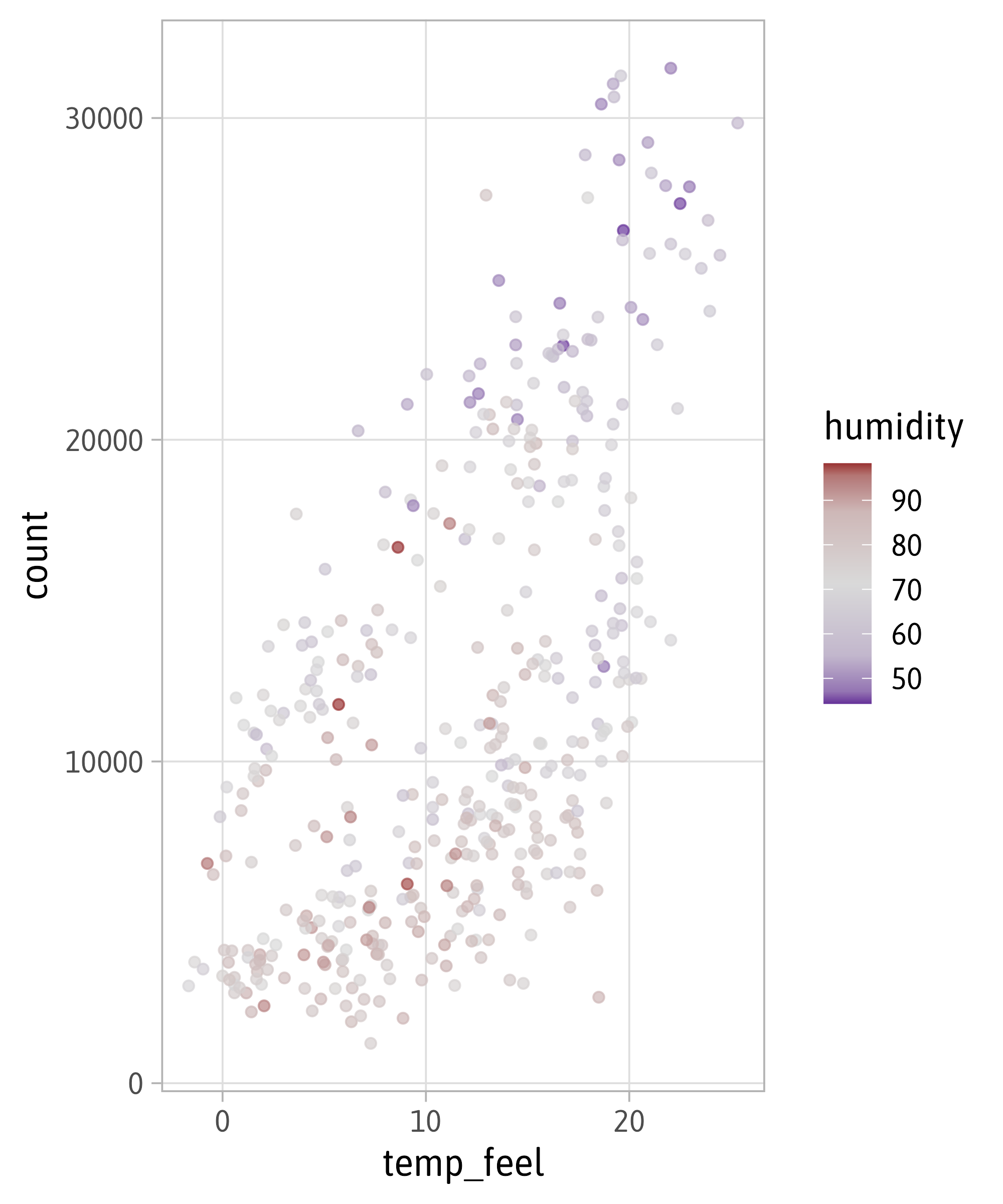
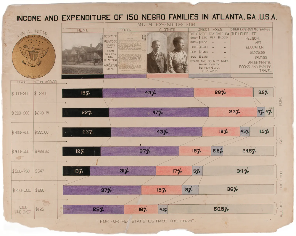
Illustration by W. E. B. Du Bois, Courtesy Library of Congress
Build Custom Color Scales
Build Custom Color Scales

Build Custom Color Scales: Categorical
Build Custom Color Scales: Categorical
Use Your Custom Color Scales: Categorical
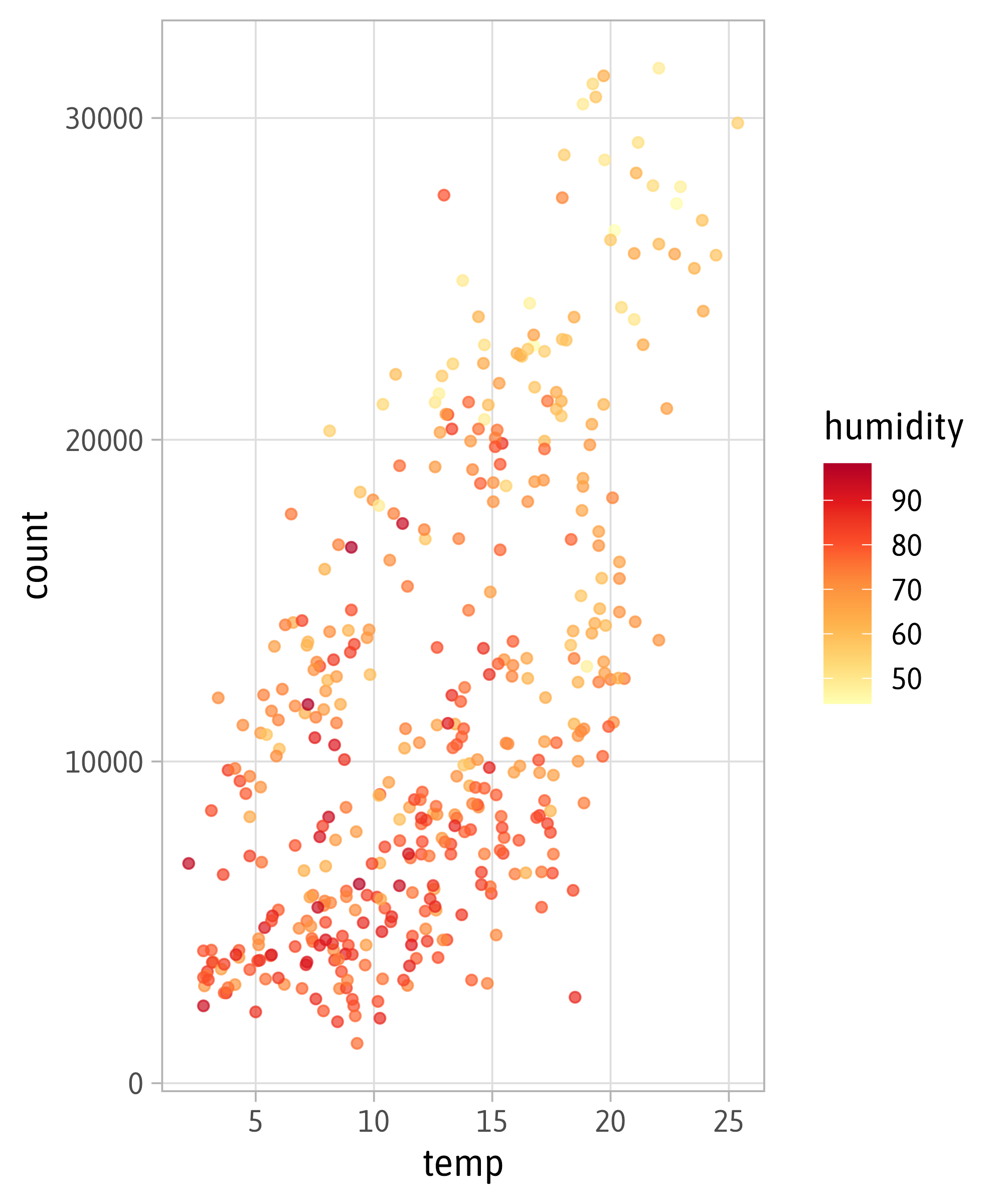
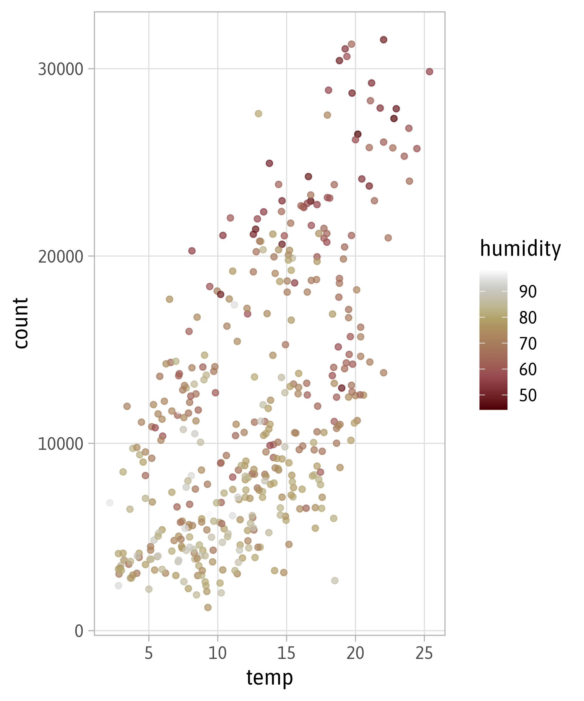
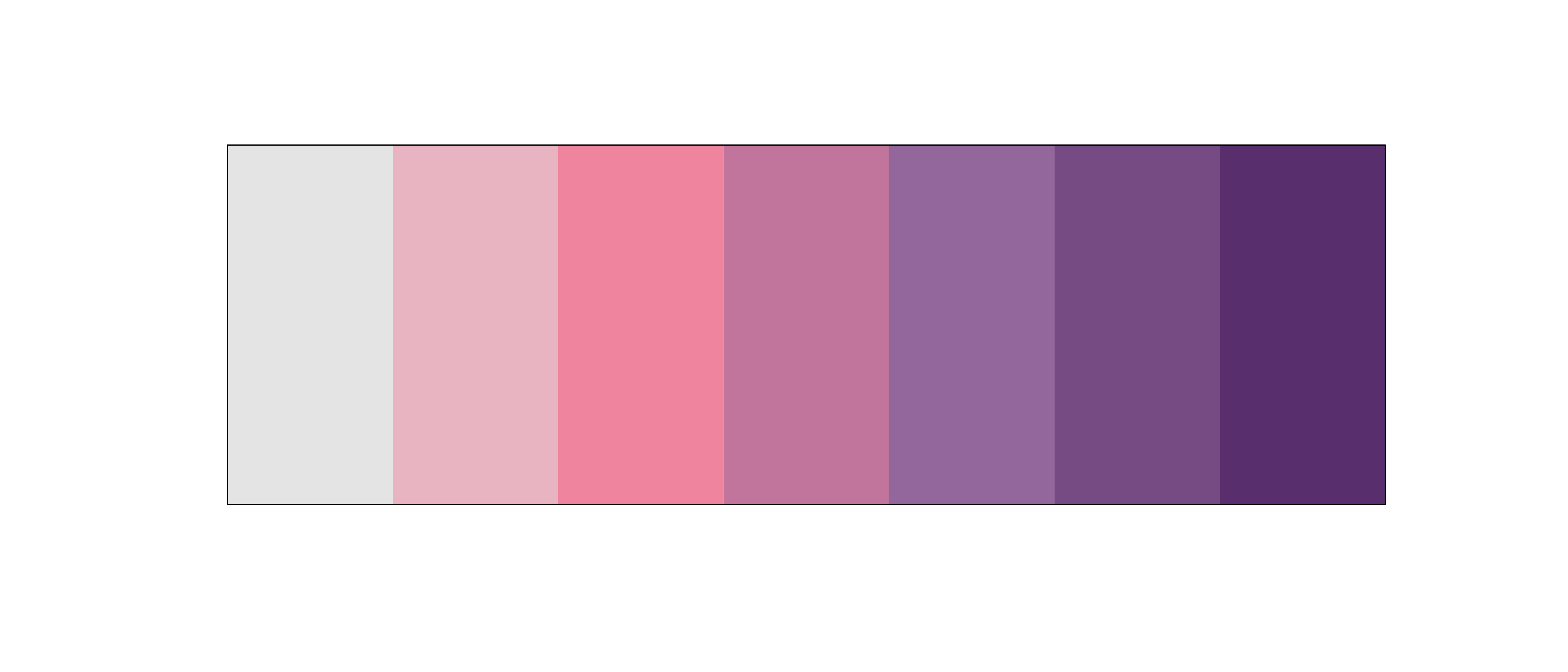
Build Custom Color Scales: Sequential
Build Custom Color Scales: Sequential
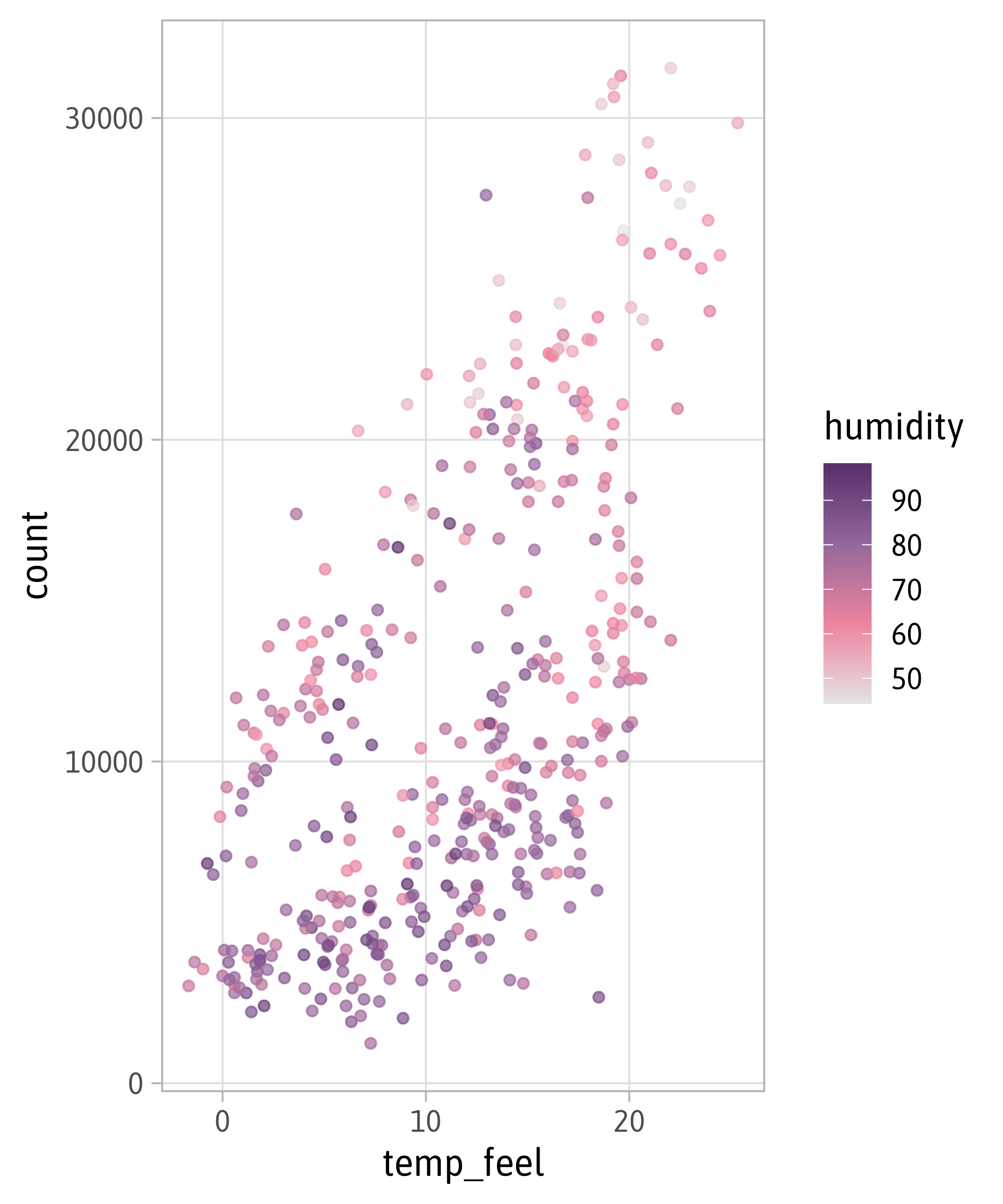
Use Your Custom Color Scales: Sequential
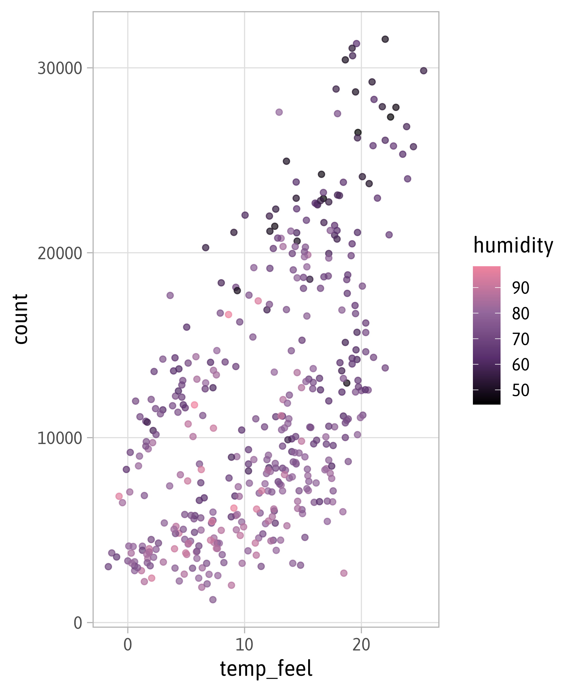
Use Your Custom Color Scales: Sequential
Evaluate HCL Spectrum
More on how to evaluate color palettes: HCLwizard and colorspace.

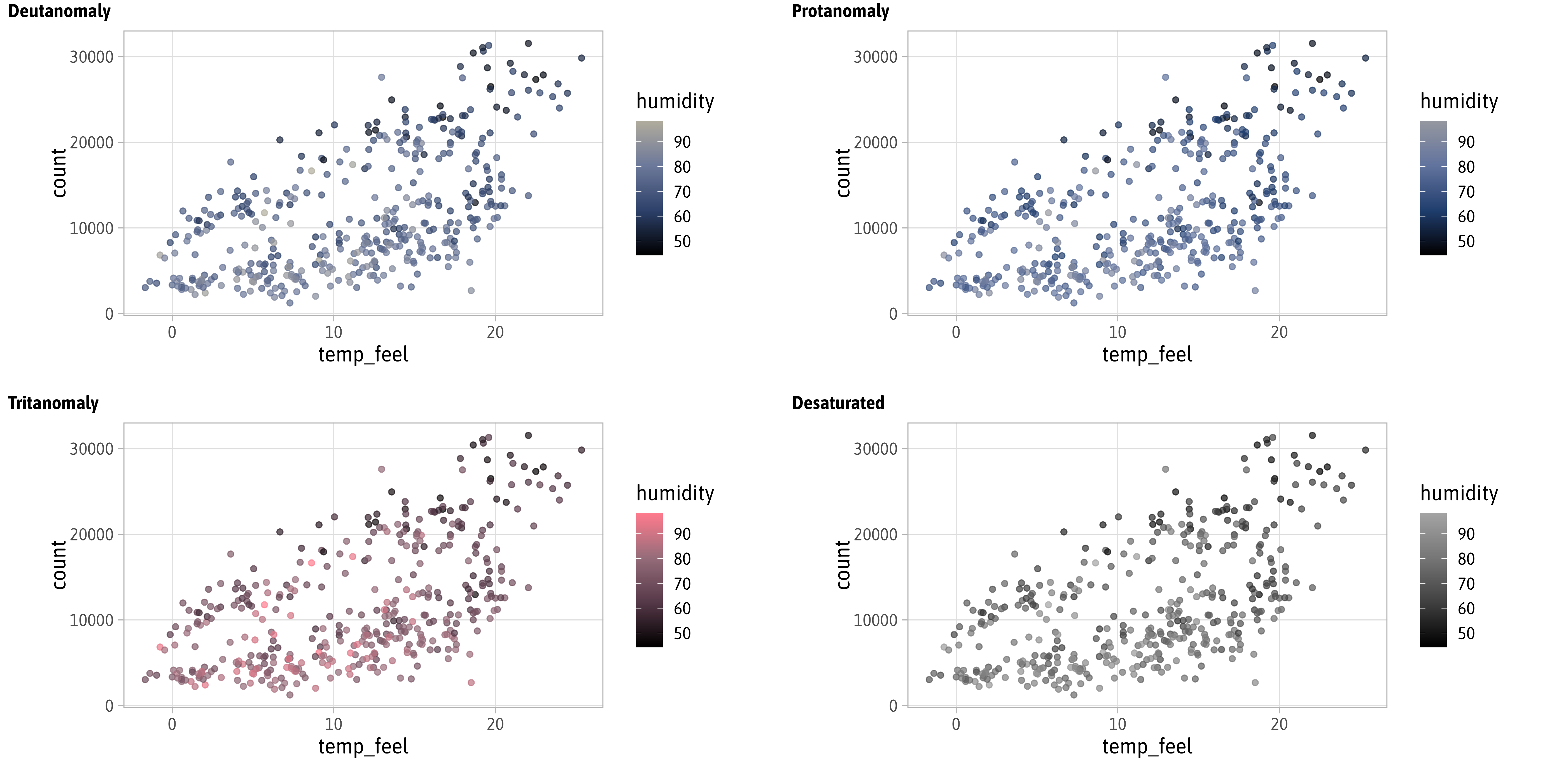
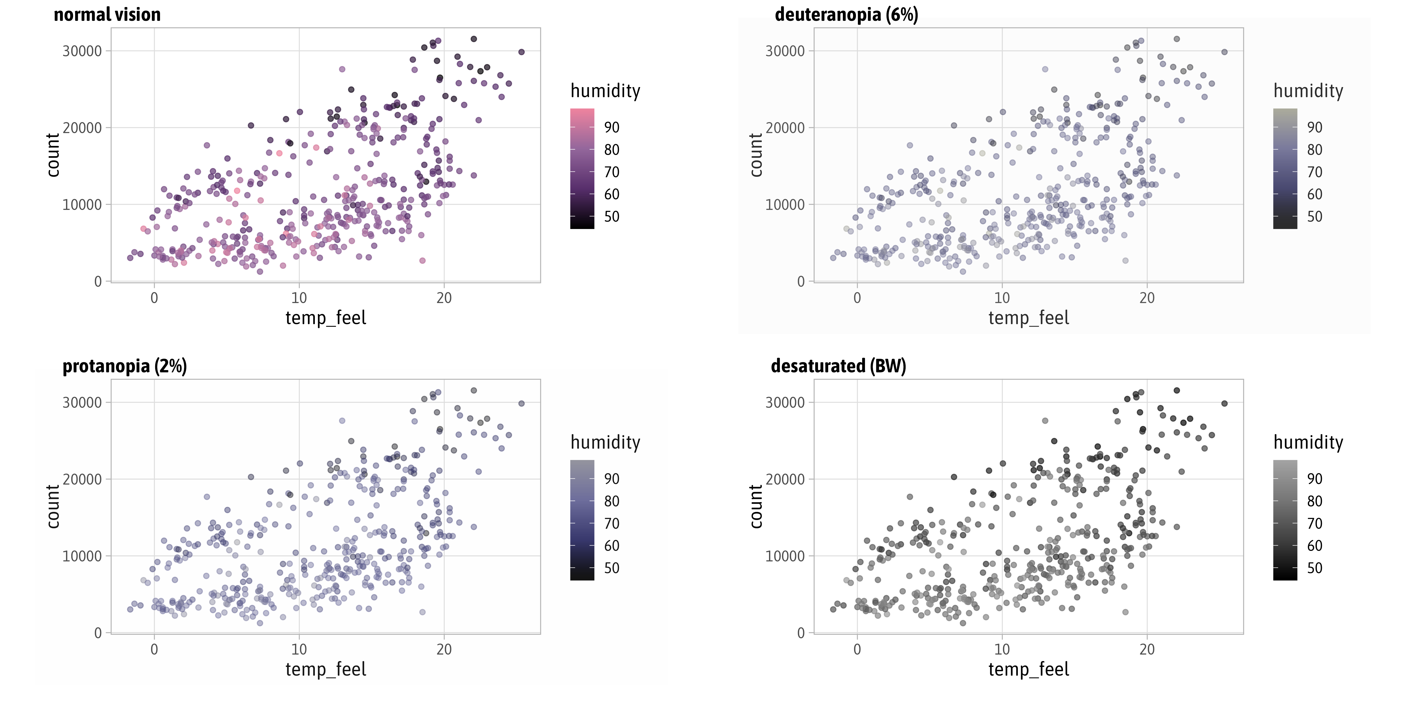
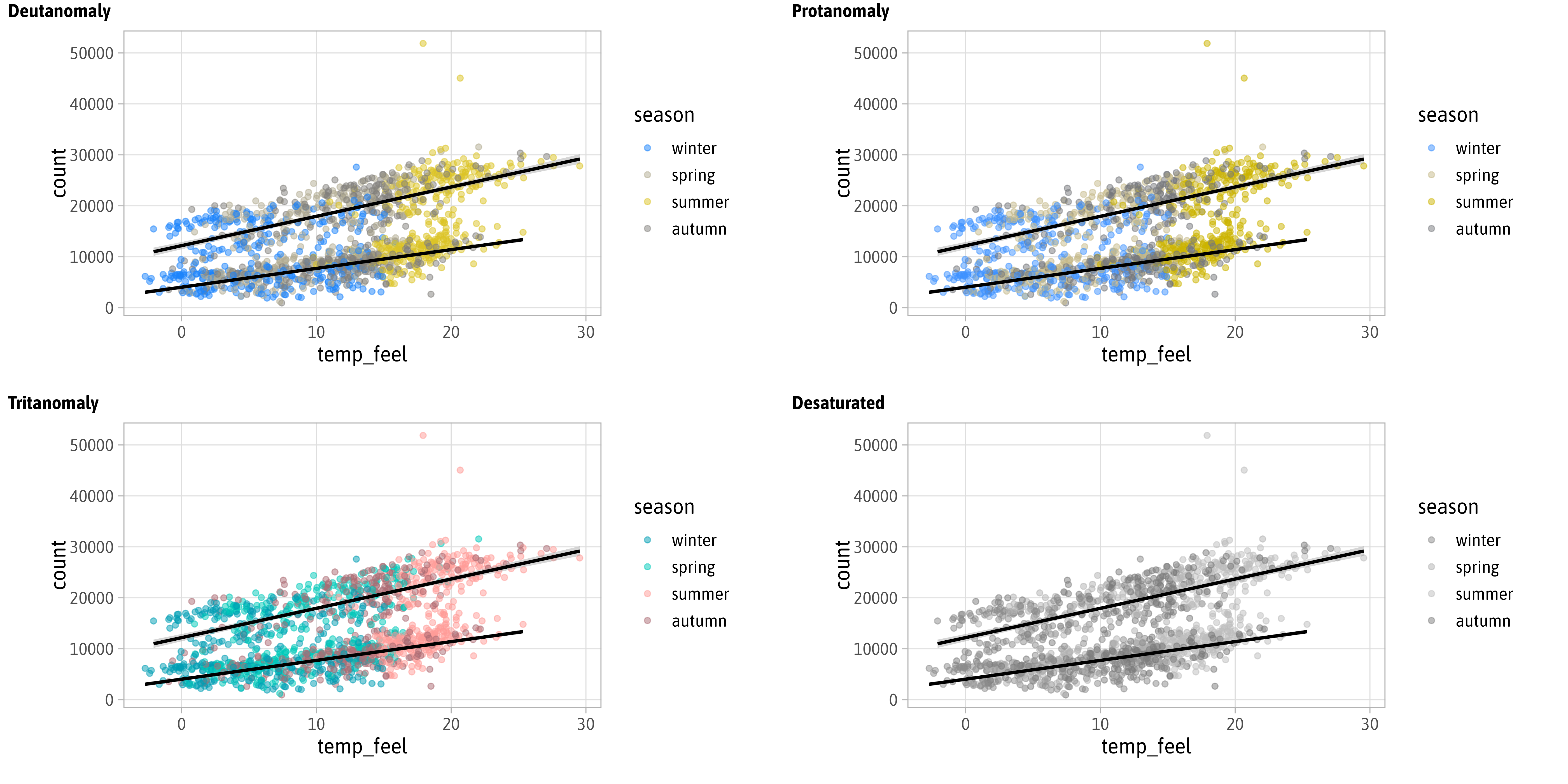
Emulate CVD
Emulate CVD

Emulate CVD
Emulate CVD
Emulate CVD

Emulate CVD
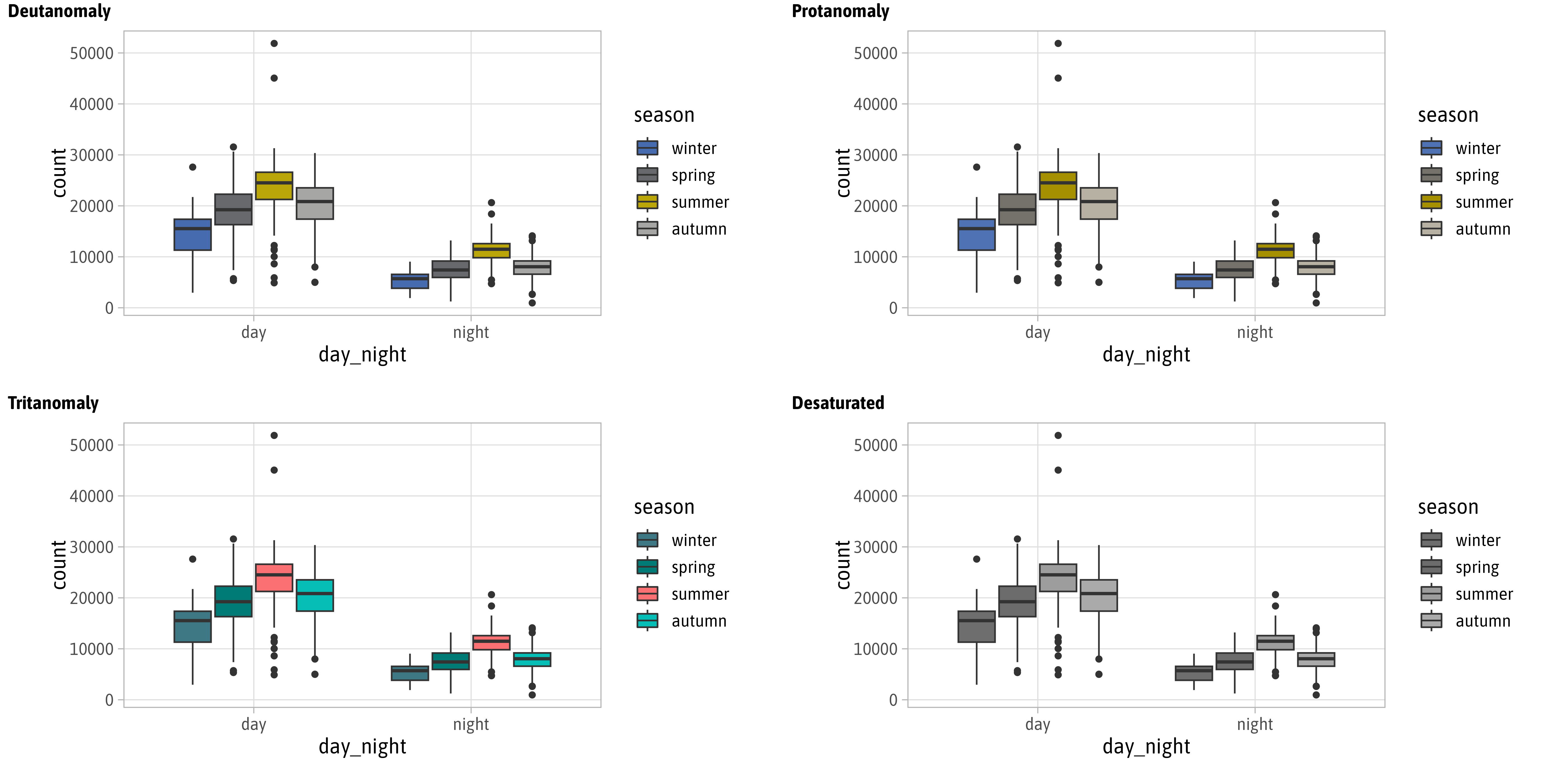
Emulate CVD
Emulate CVD
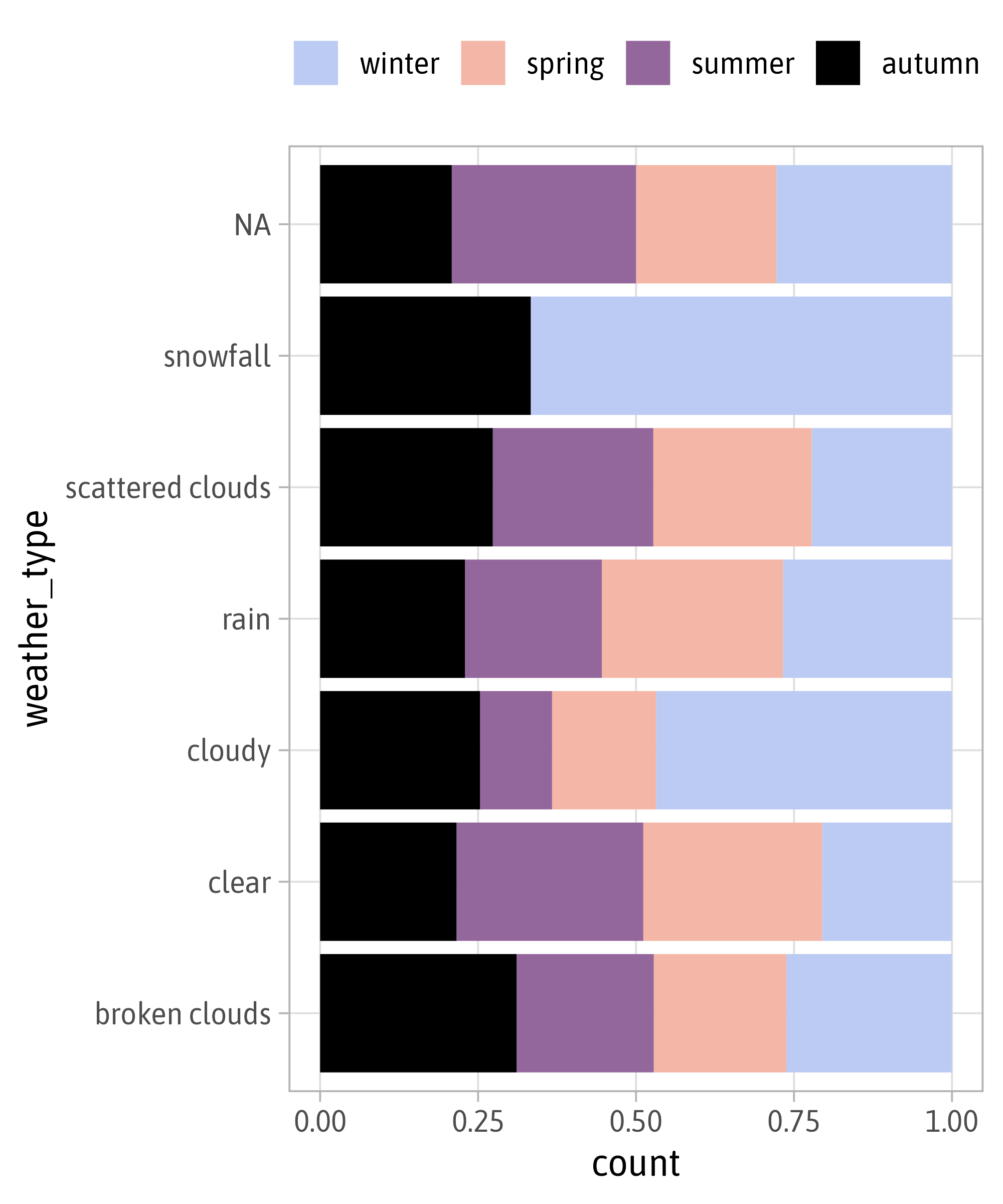
Exercise 1
- Add colors to our bar chart from the last exercise: