Engaging and Beautiful Data Visualizations with ggplot2
Fundamentals & Workflows
— Exercise Solutions —
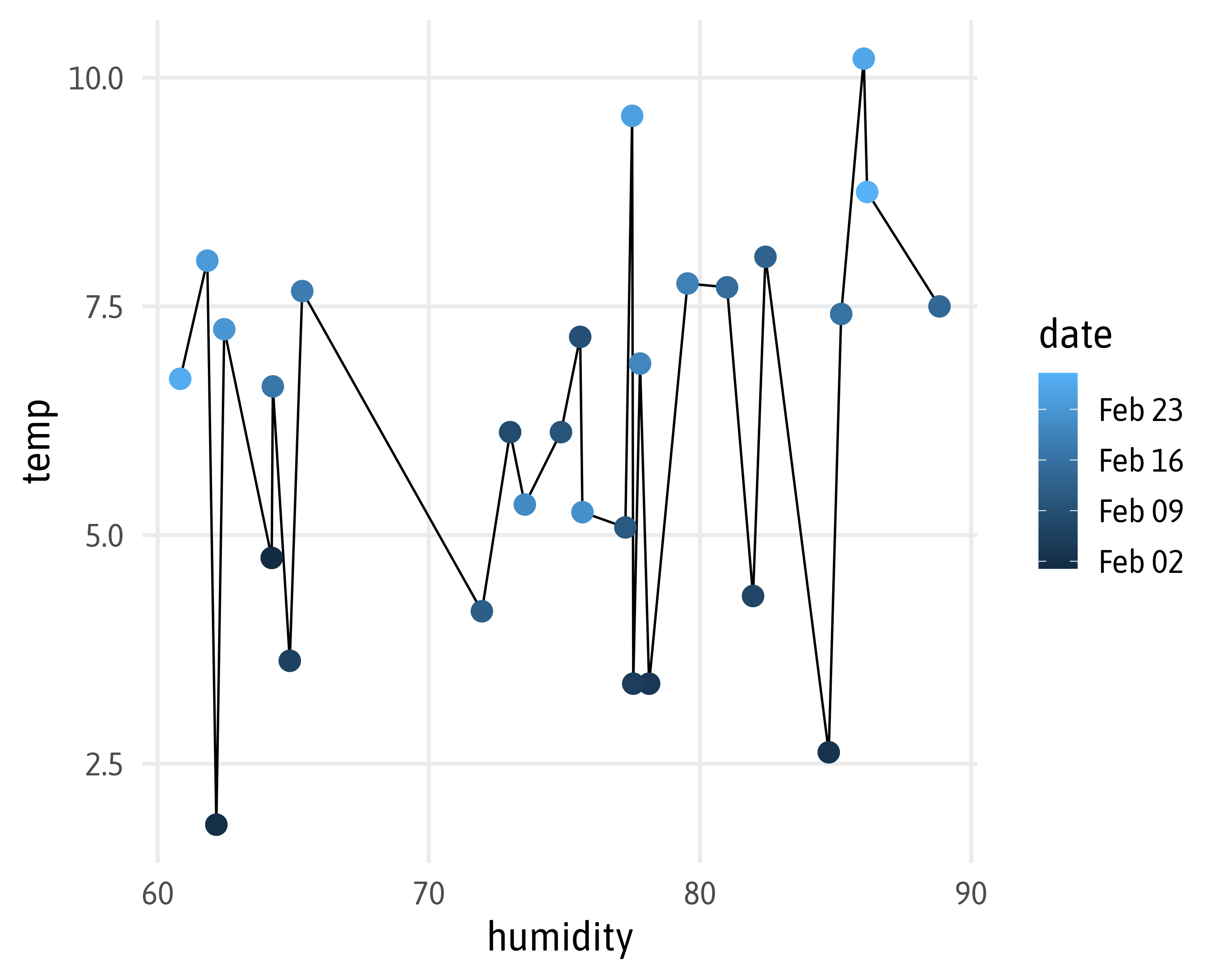
geom_line() versus geom_path()

layer()
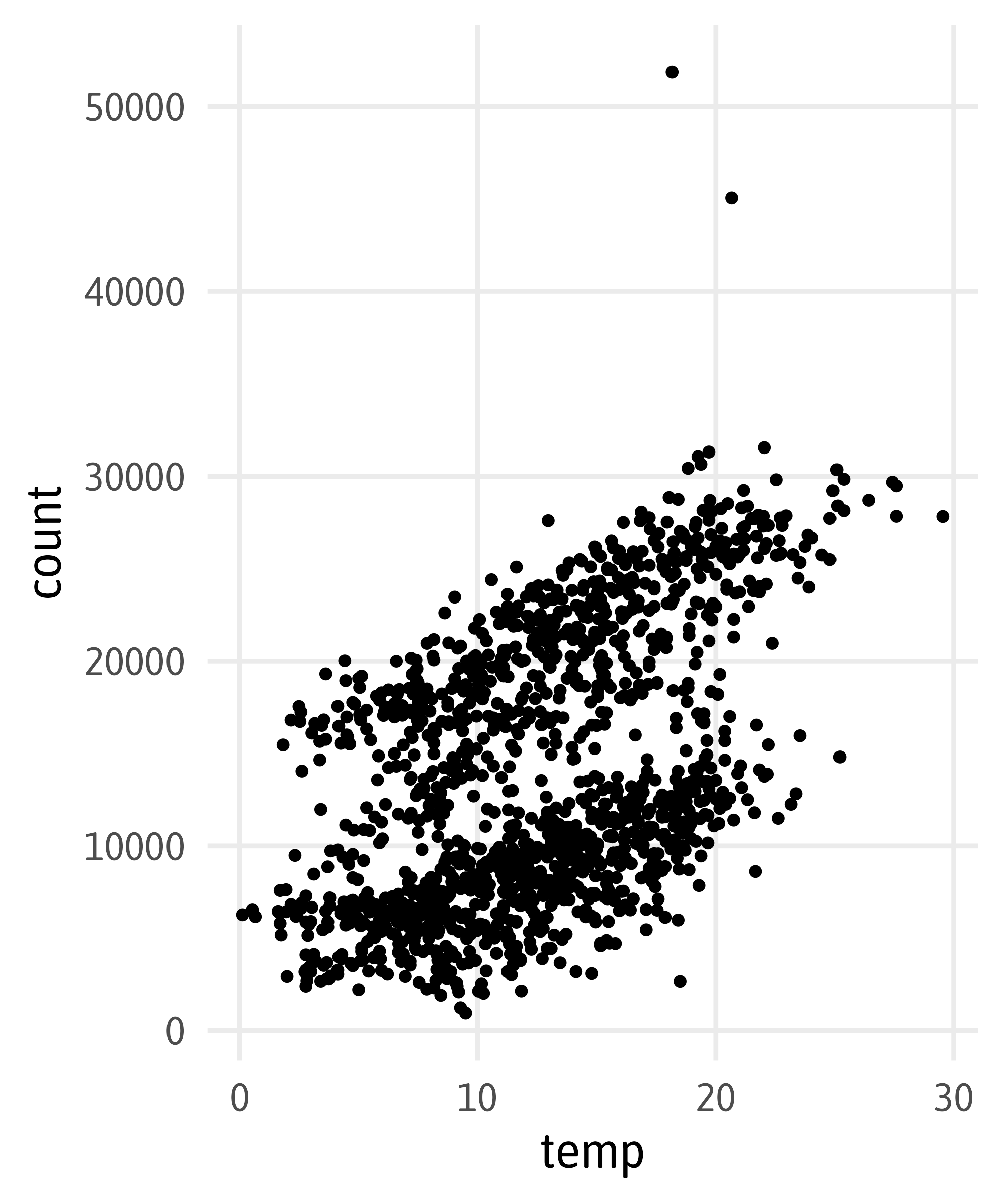
layer()

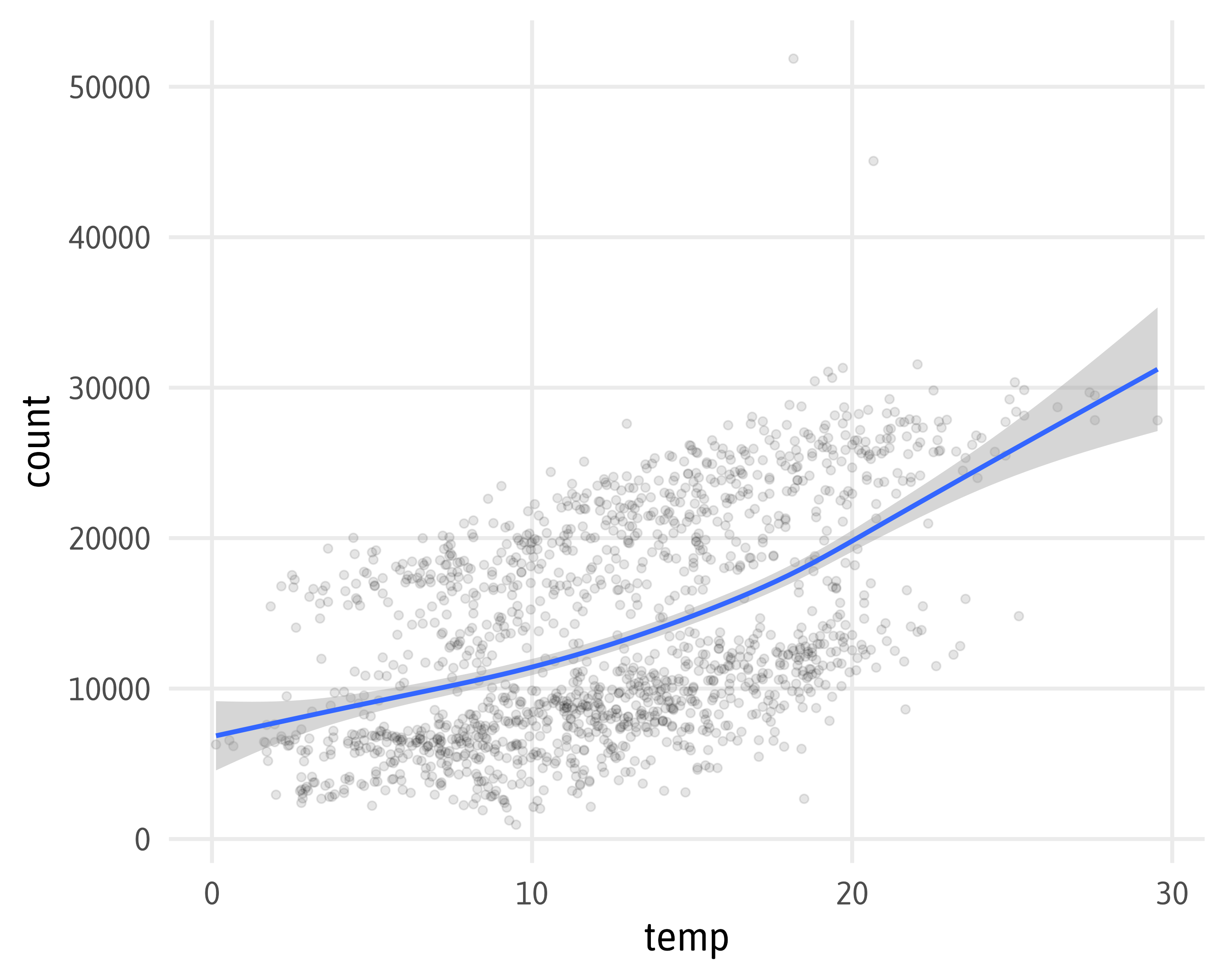
geom_smooth() and stat_smooth()

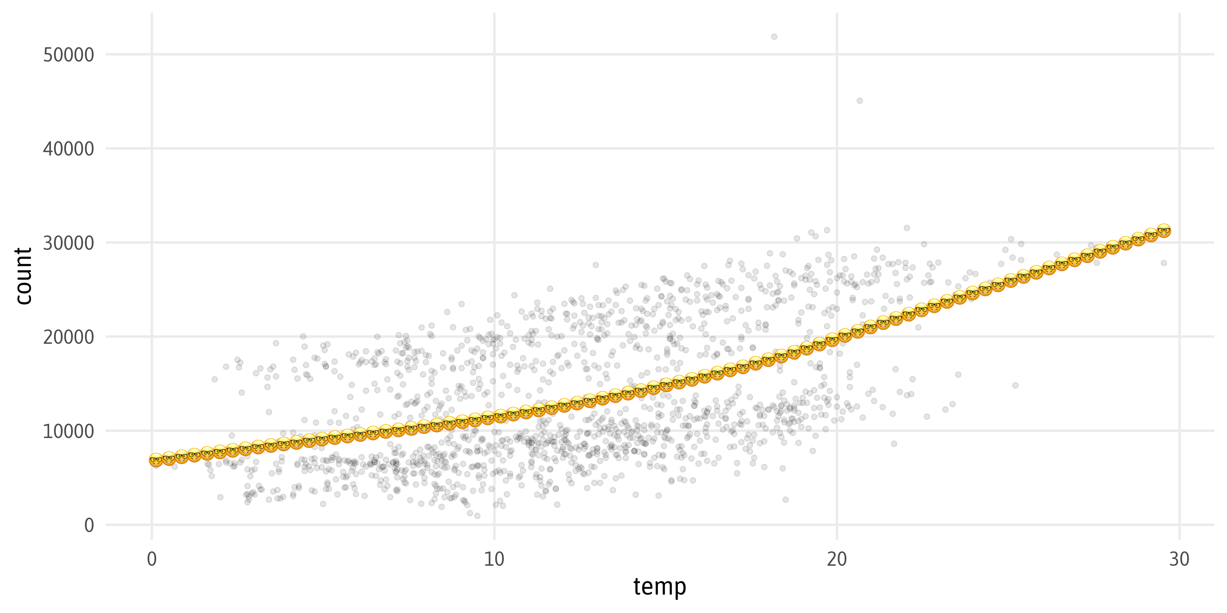
“Non-Standard Geom”
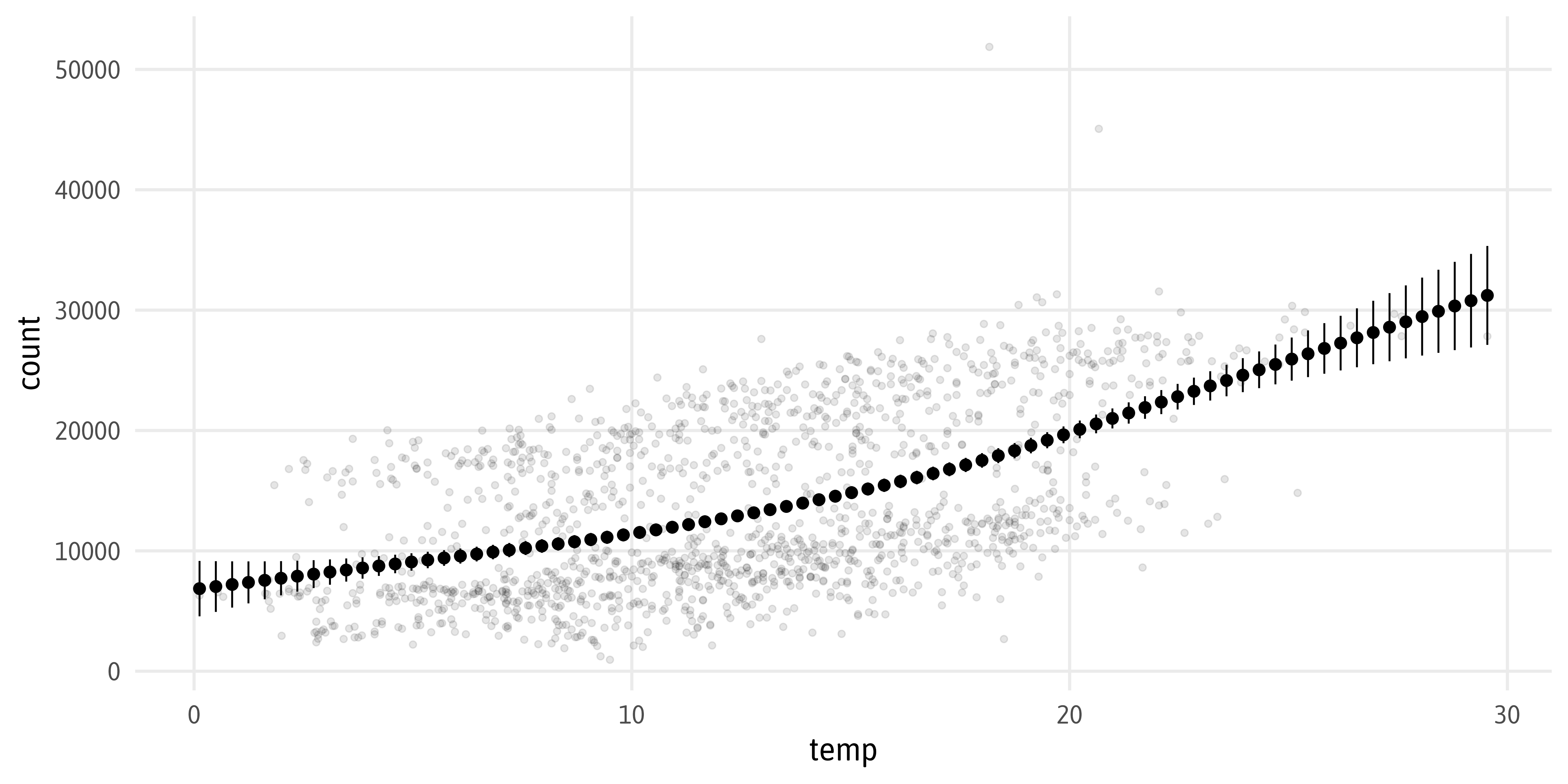
“Non-Standard Geom”
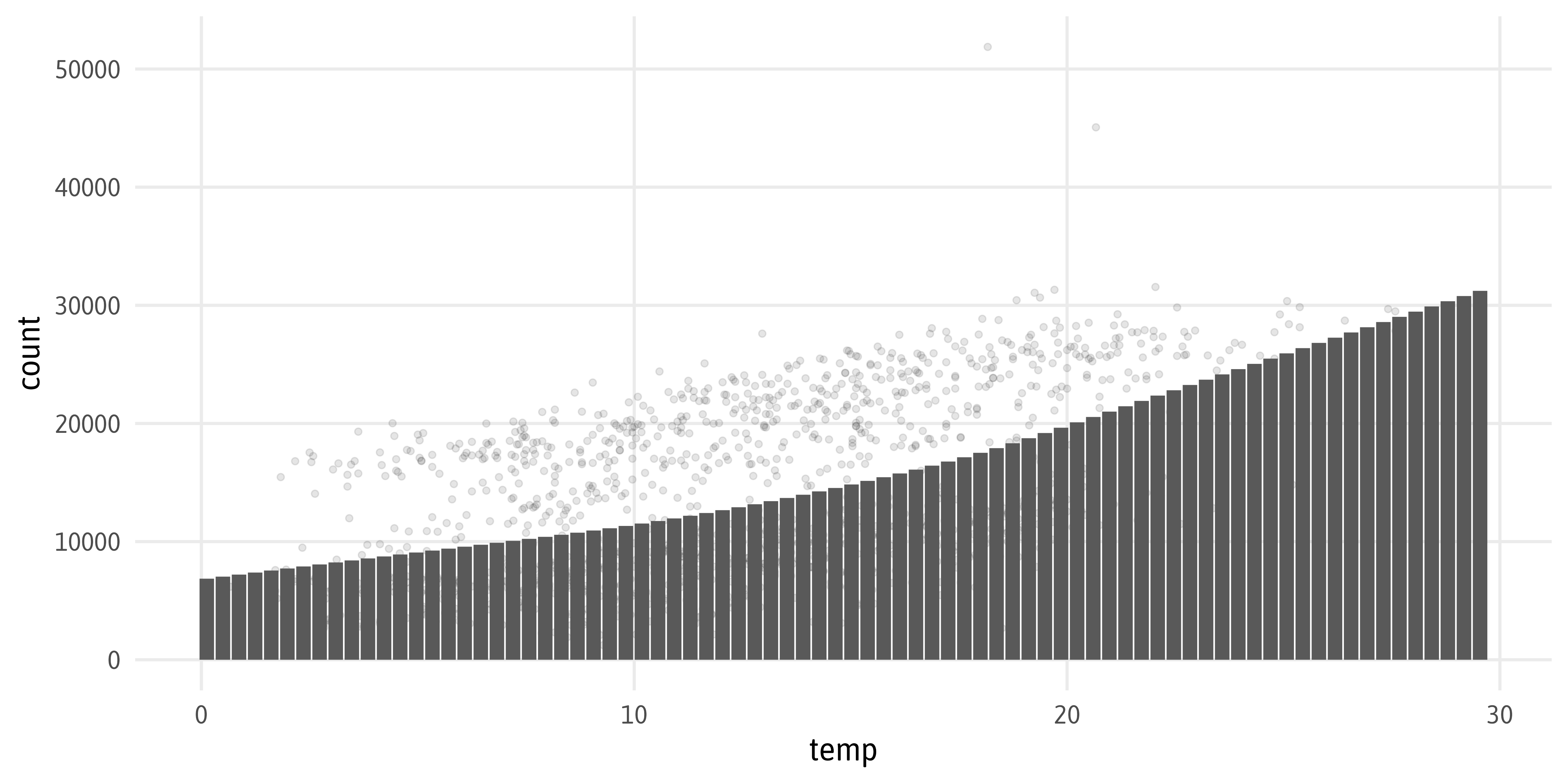
“Non-Standard Geom”
geom_* versus stat_*

geom_* versus stat_*
Remove Legends

Remove Legends: Layer
Remove Legends: Aesthetic

Remove Legends: Aesthetic

Remove Legends: All

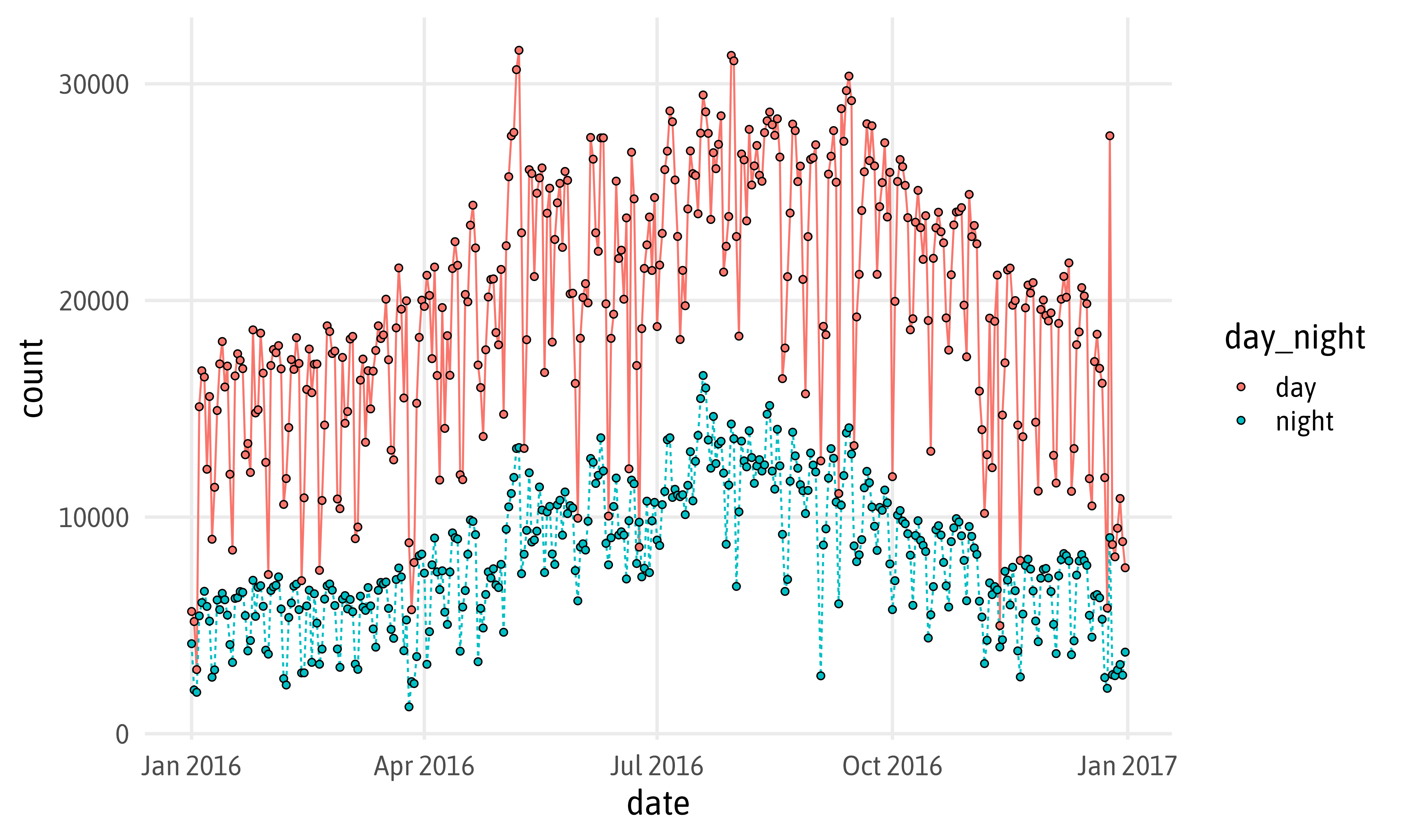
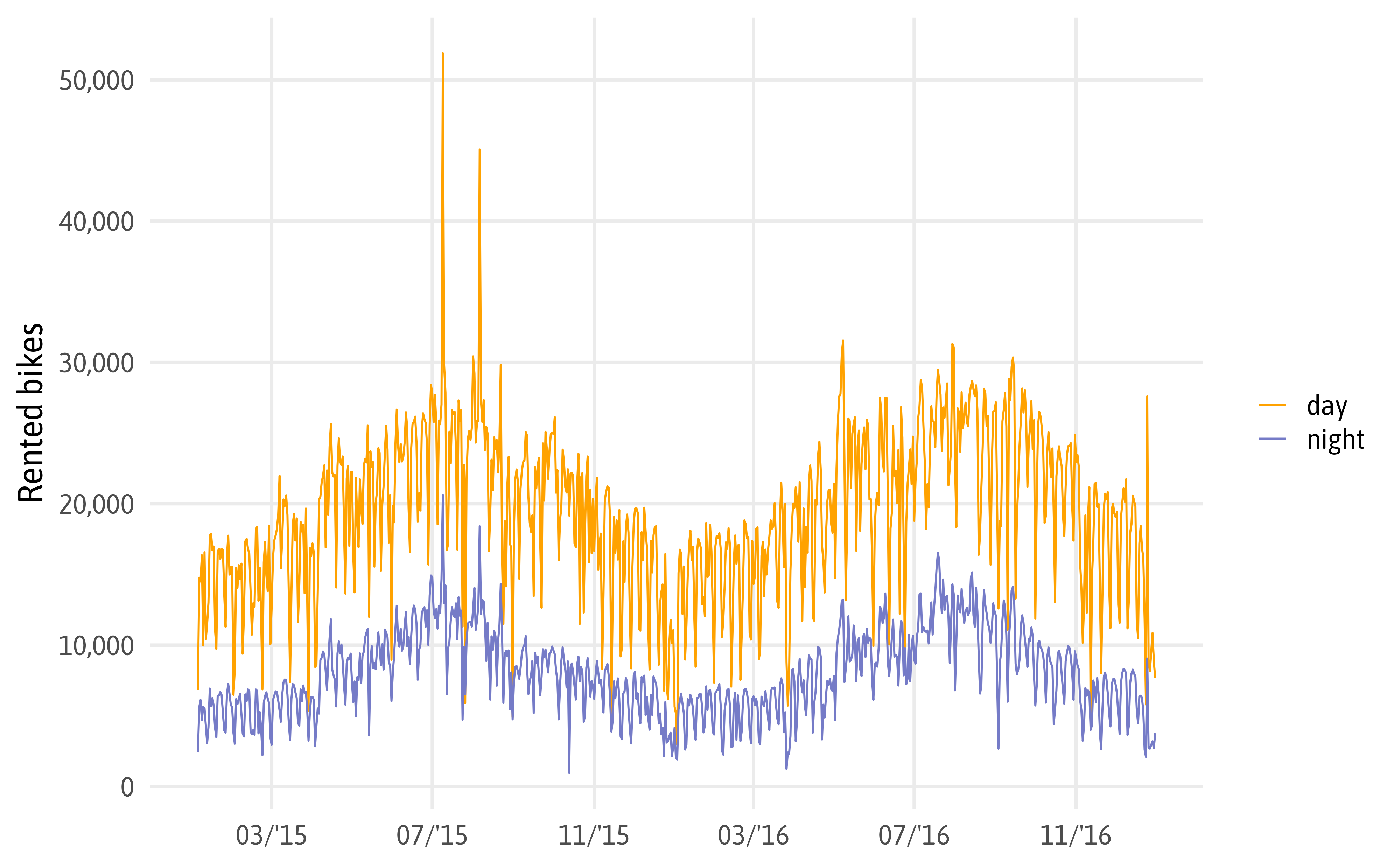
Time Series
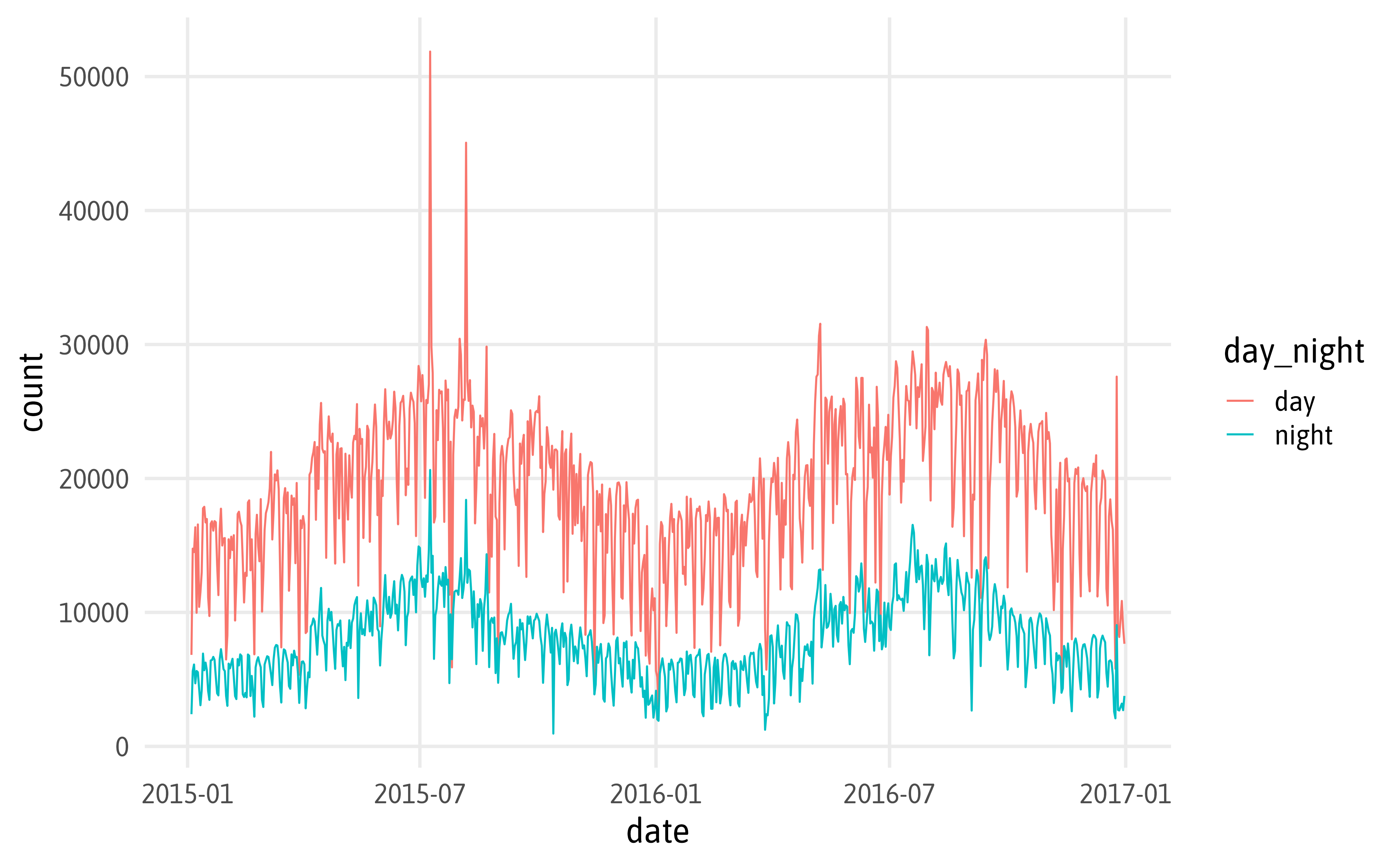
Time Series
Box and Whisker Plots
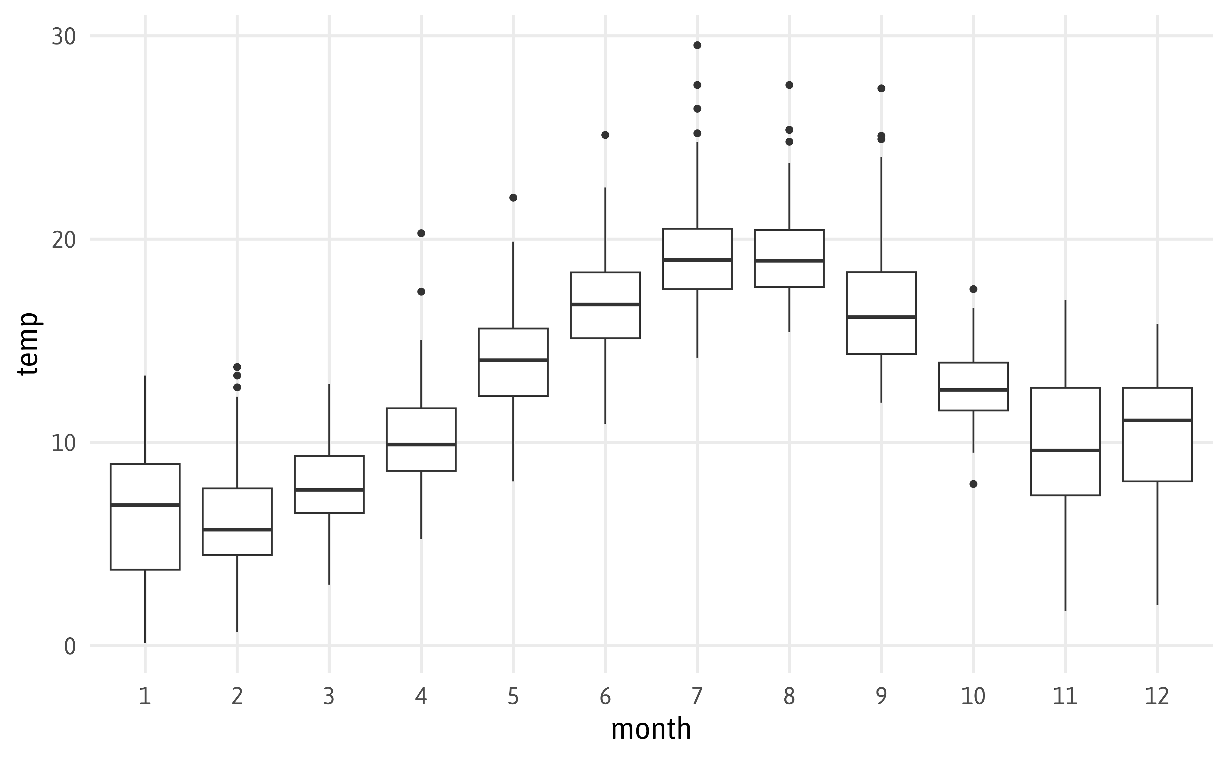
Box and Whisker Plots
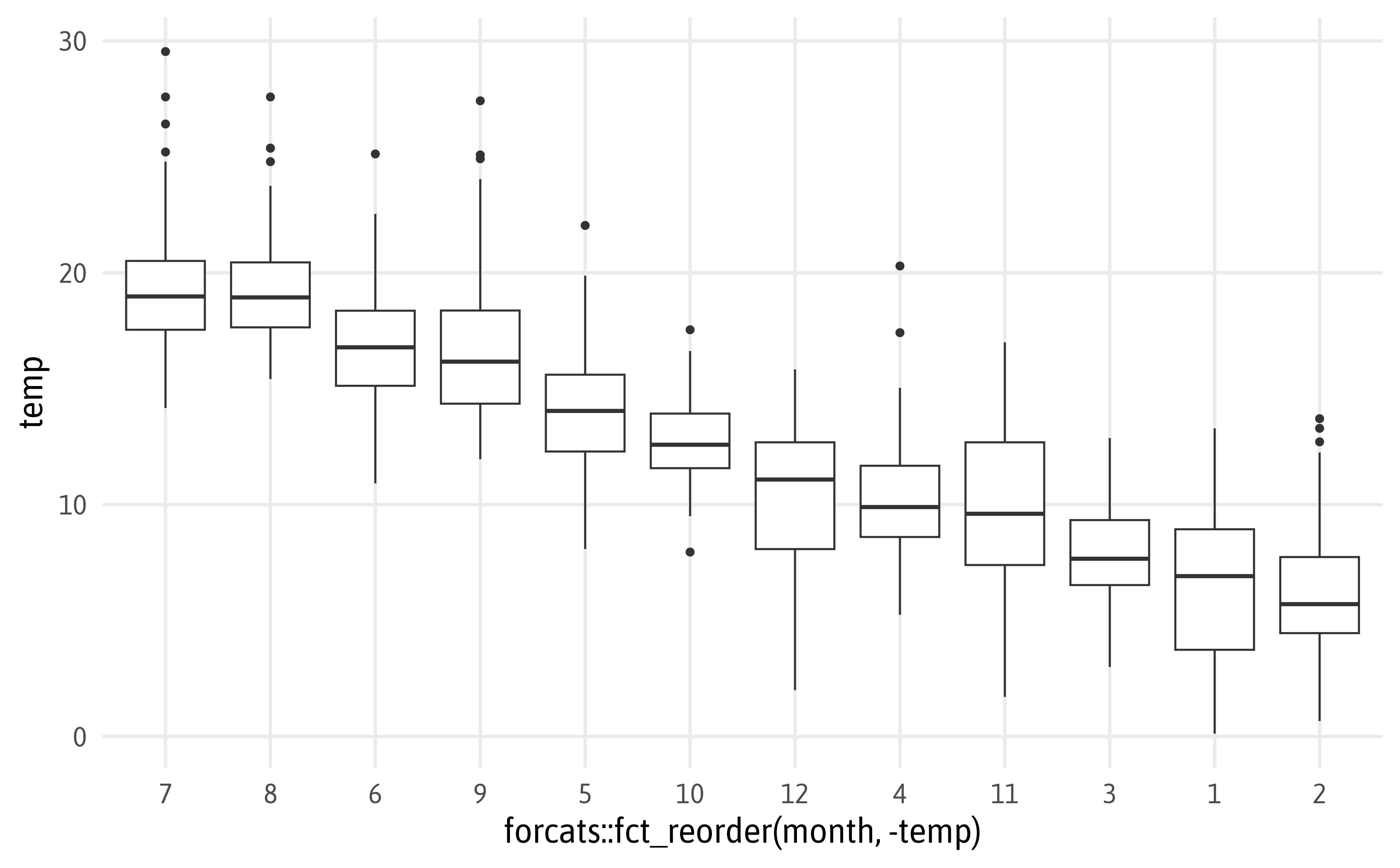
Box and Whisker Plots

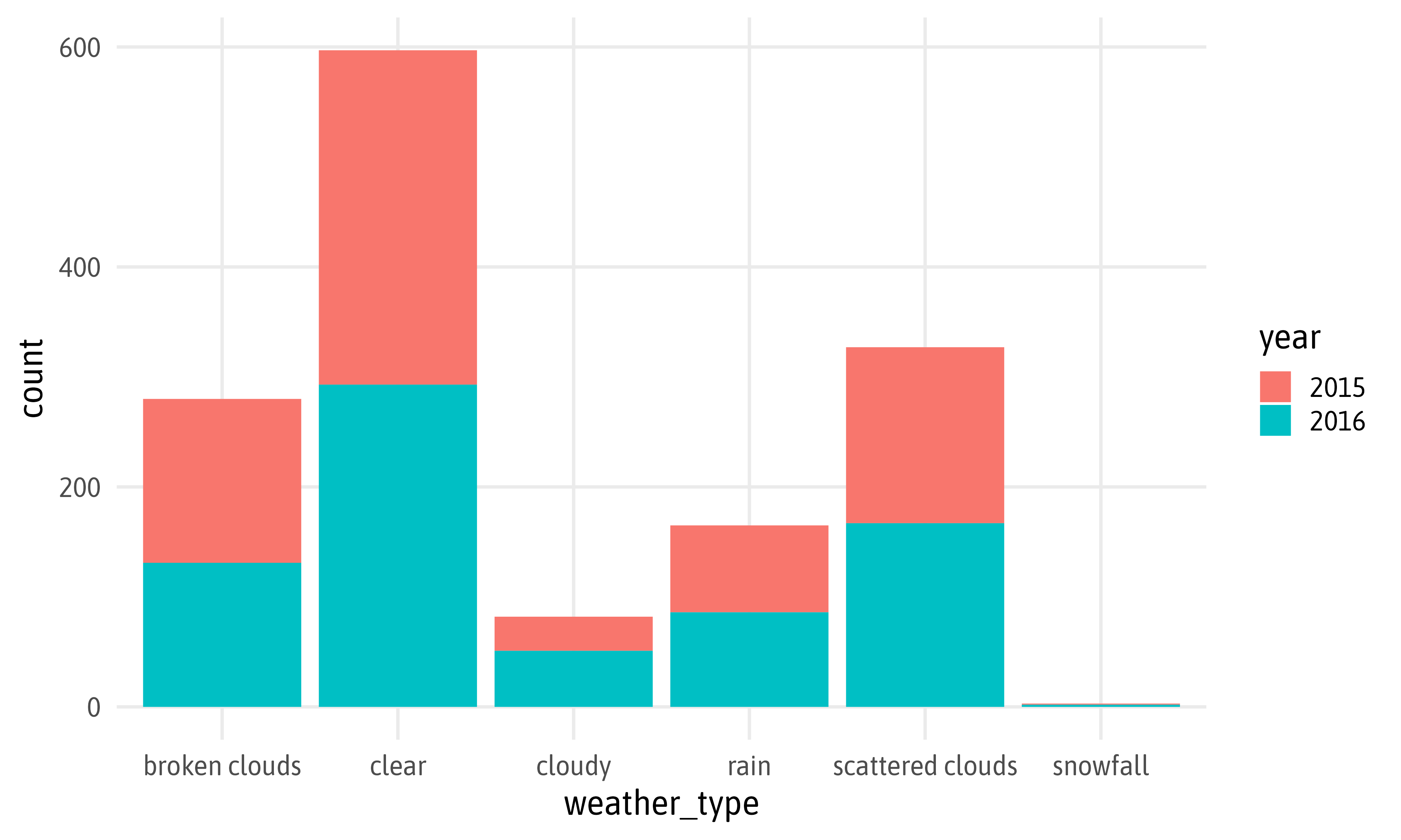
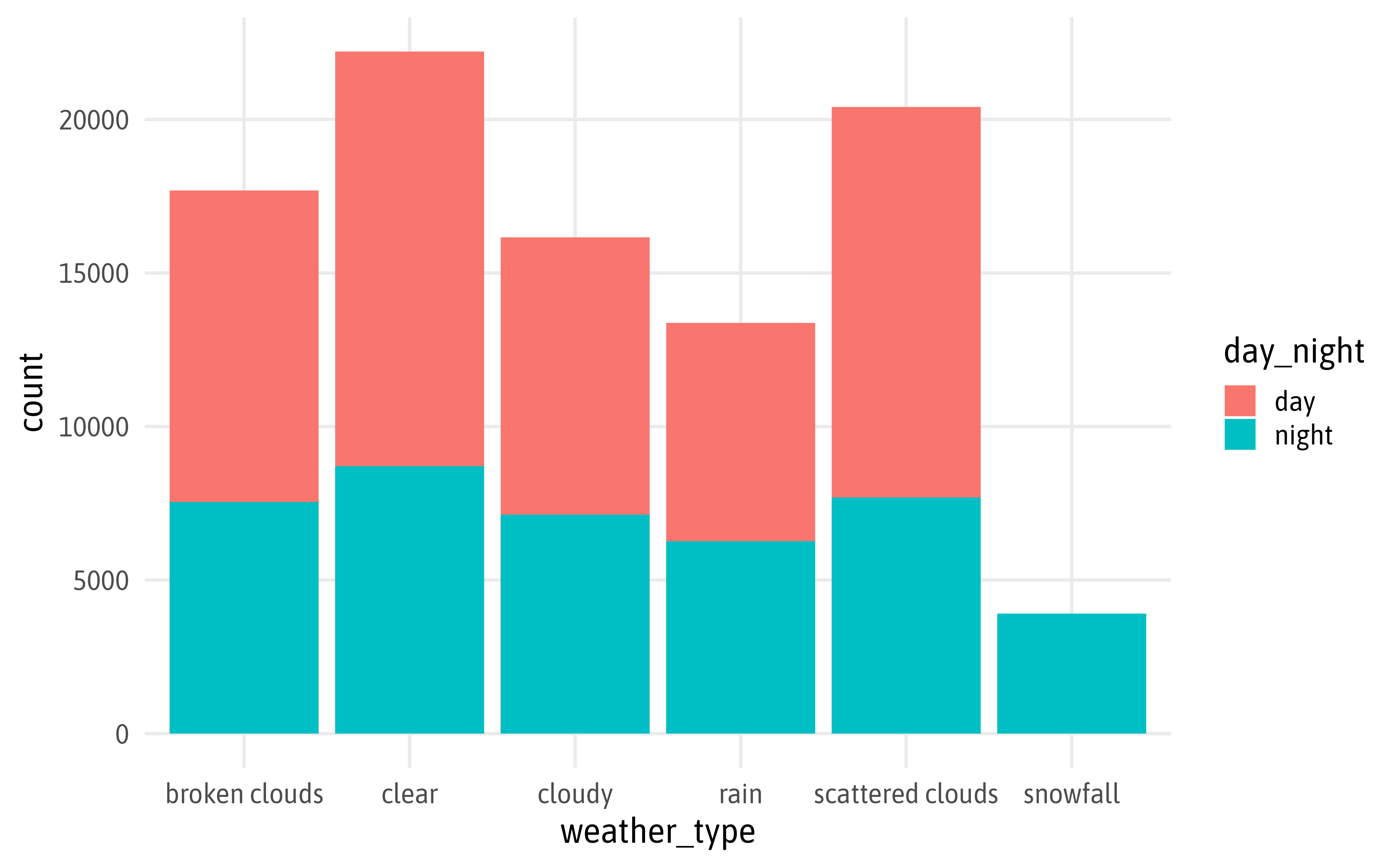
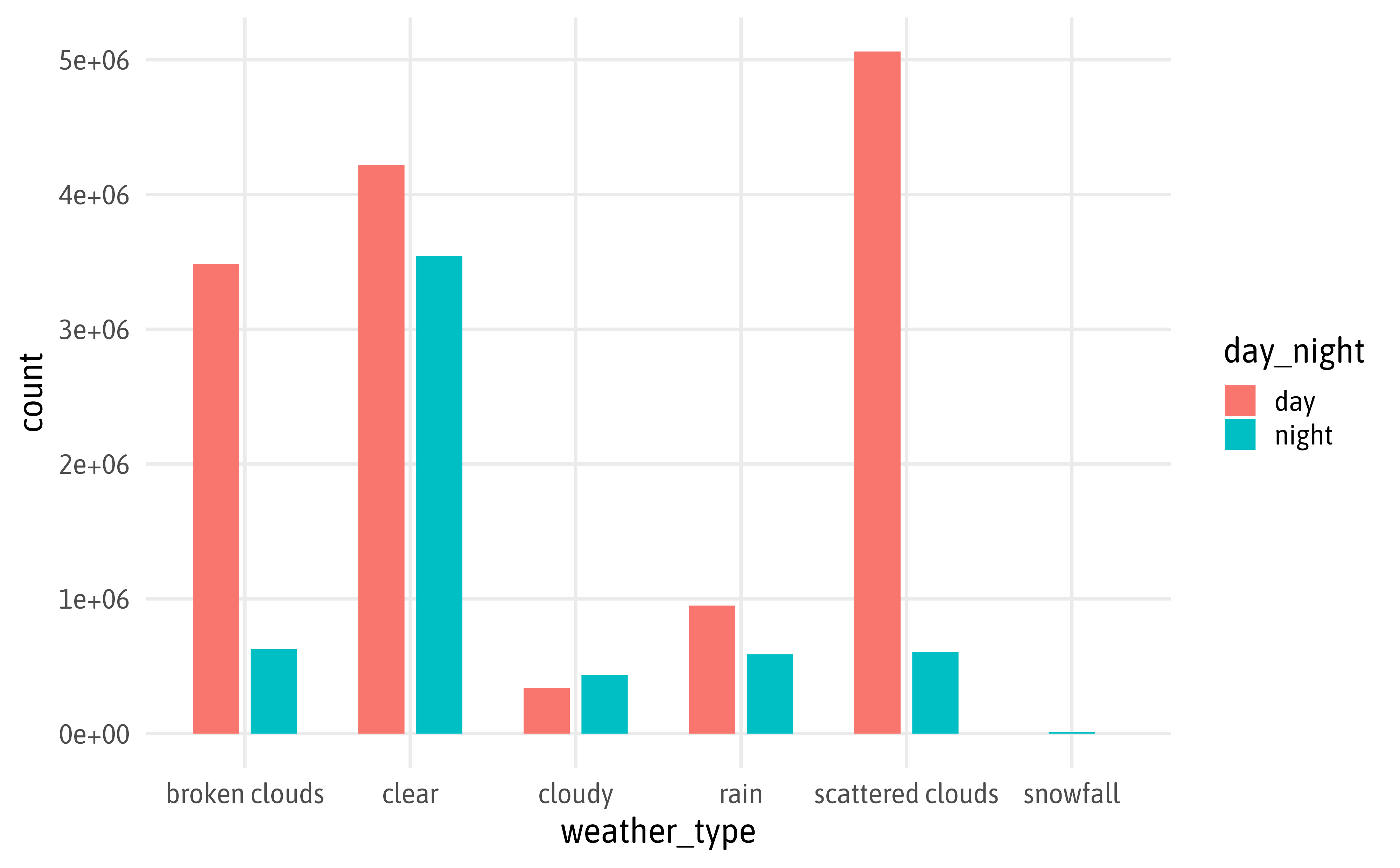
Bar Chart

Bar Chart
Bar Chart
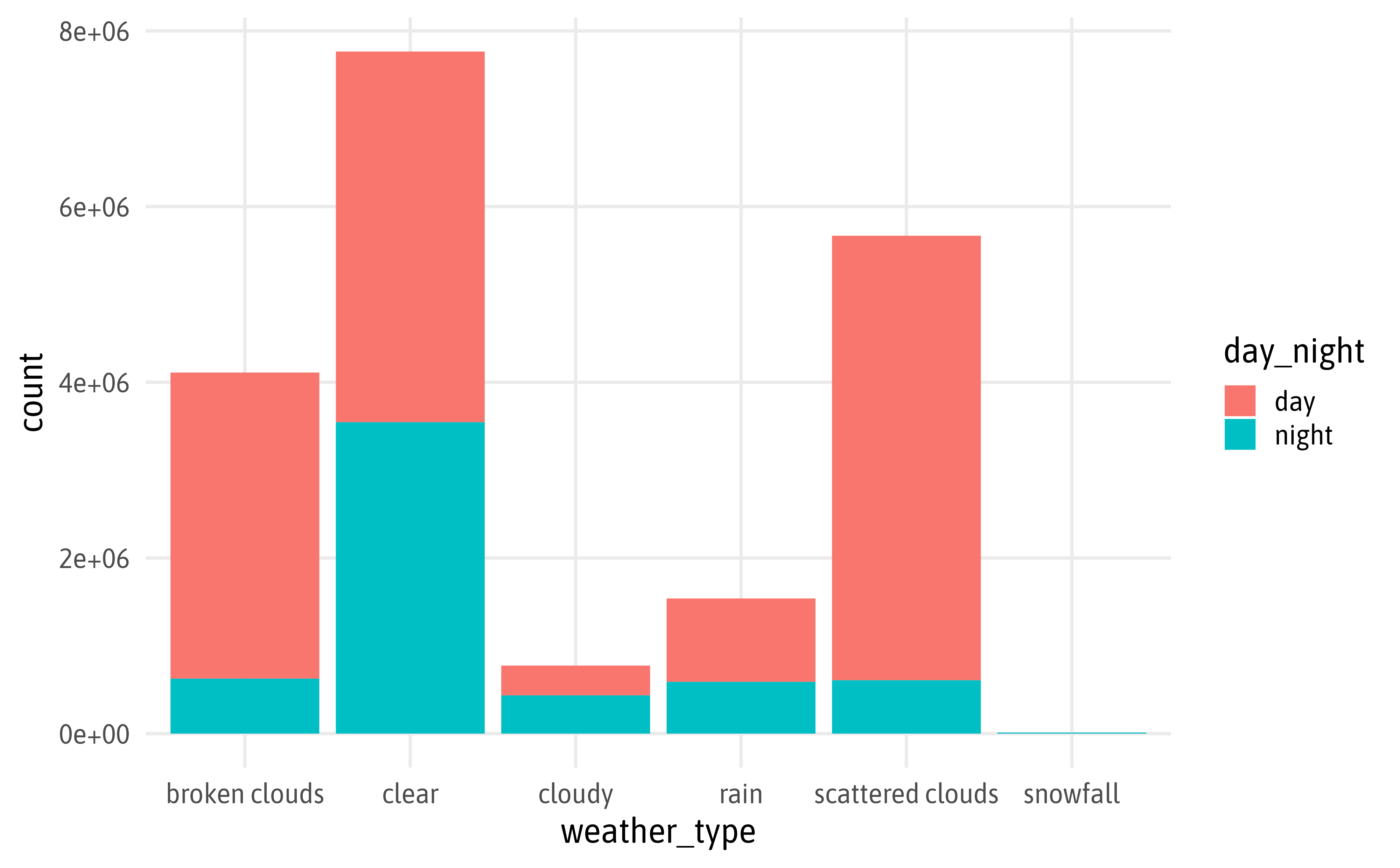
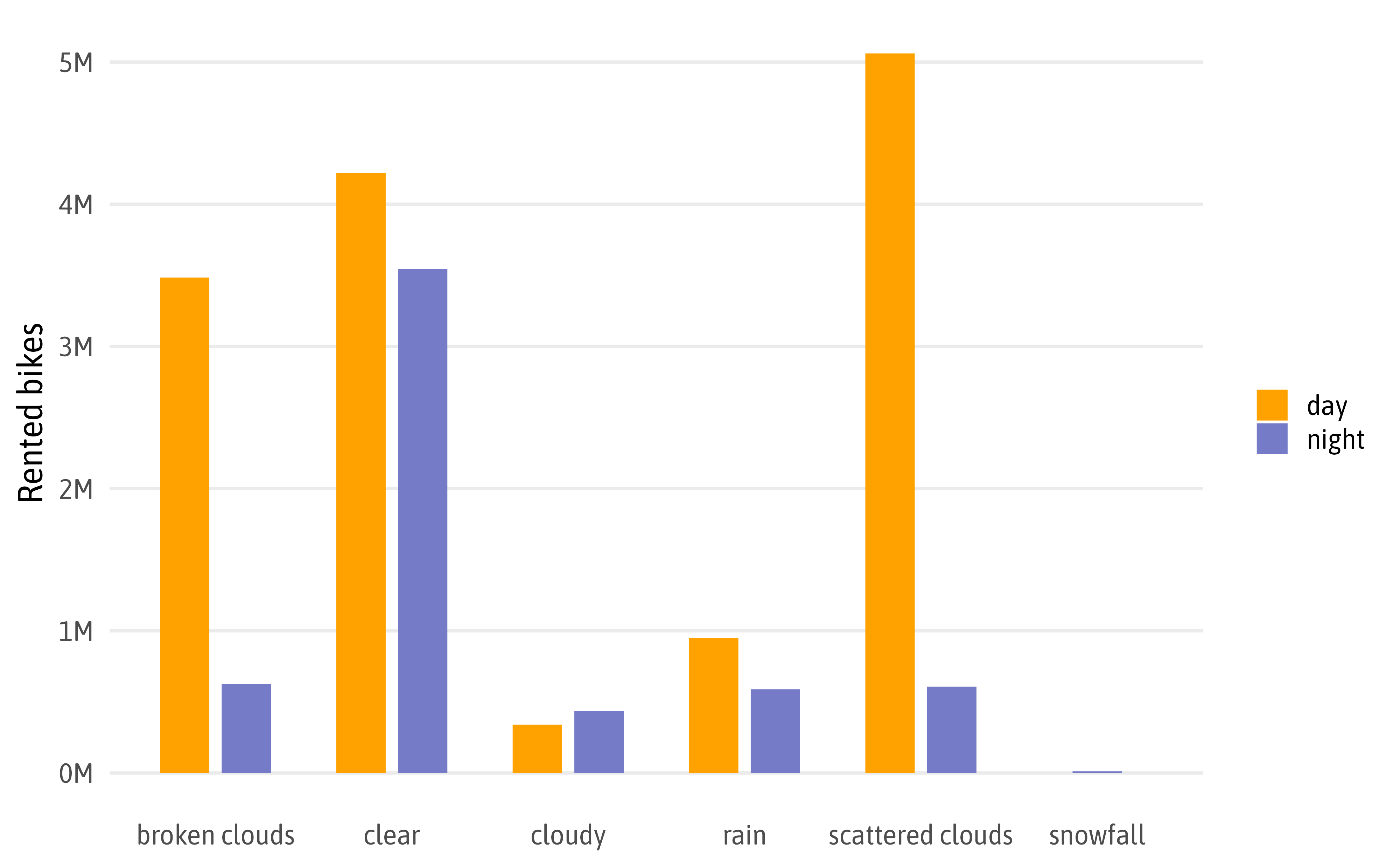
Bar Chart

Bar Chart
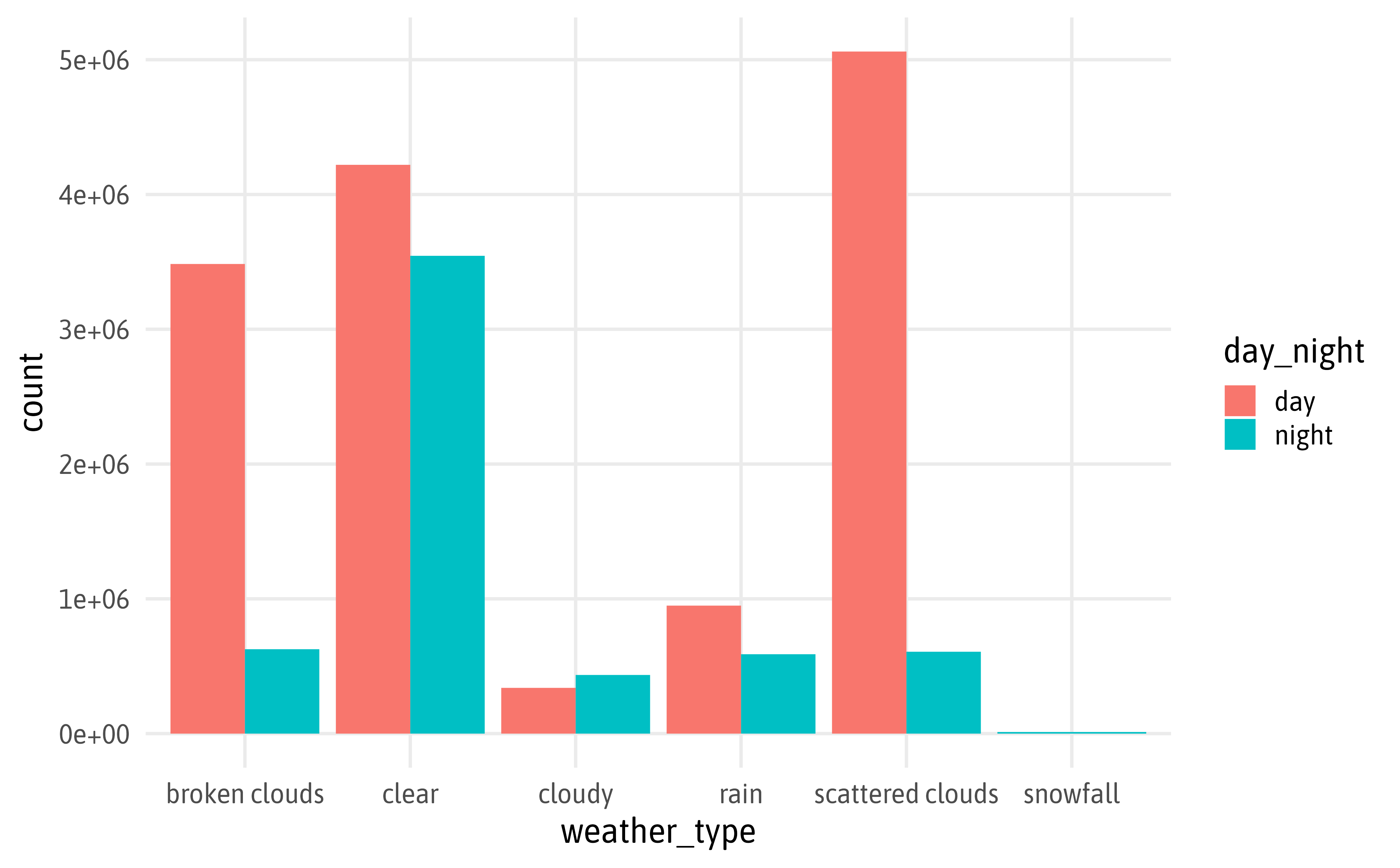
Bar Chart
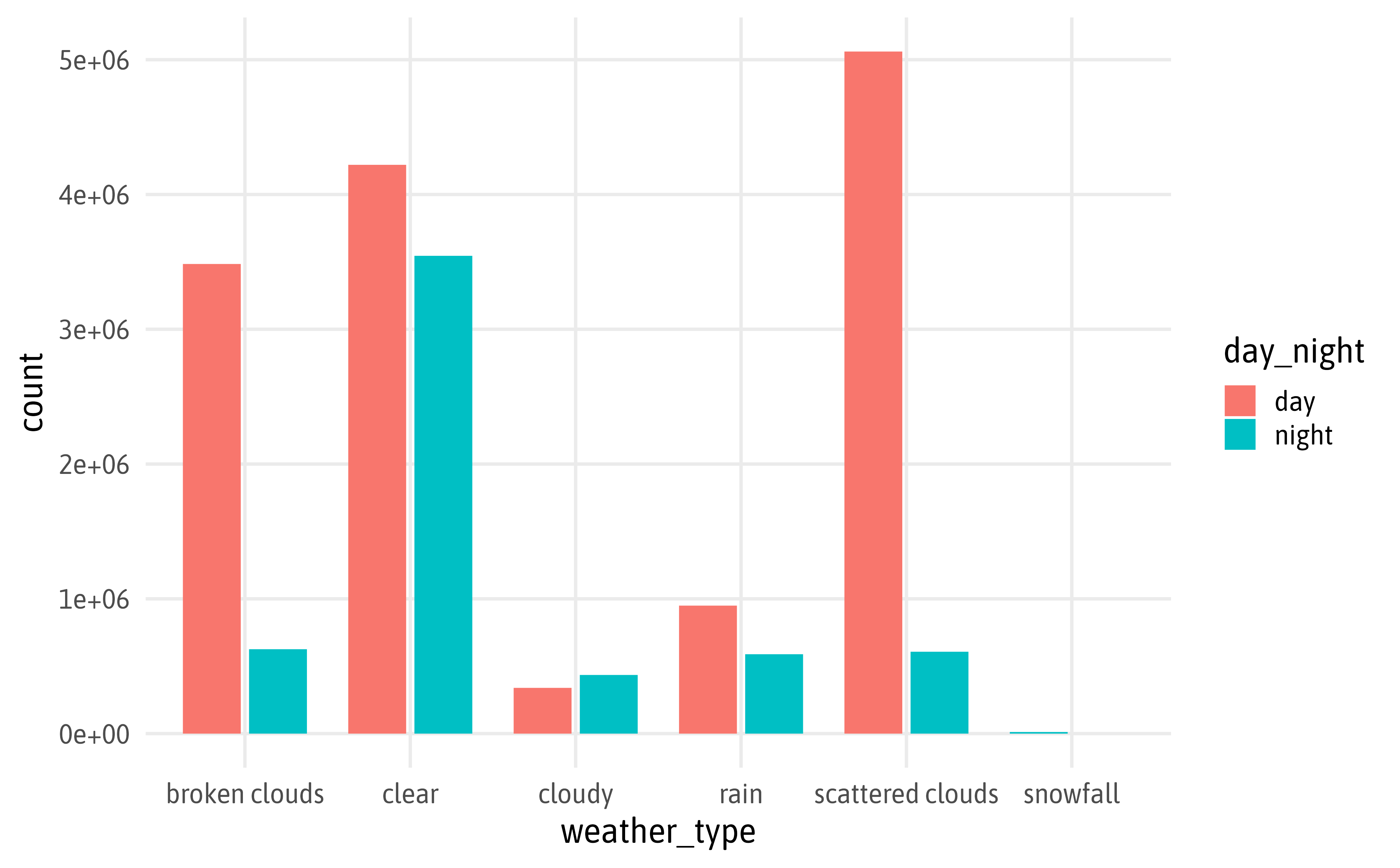
Bar Chart
Bar Chart
Combine Plots
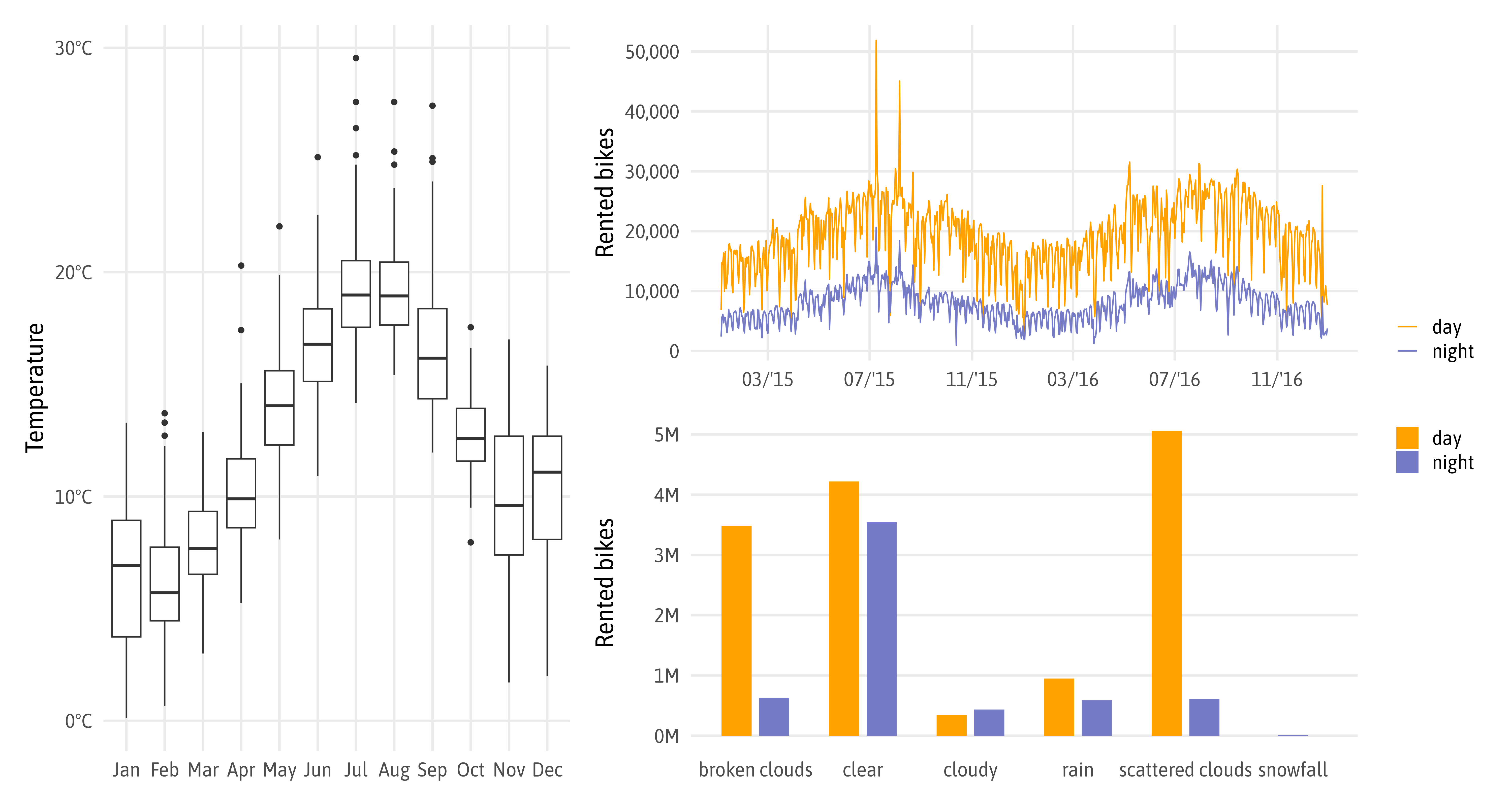
Combine Plots

Combine Plots
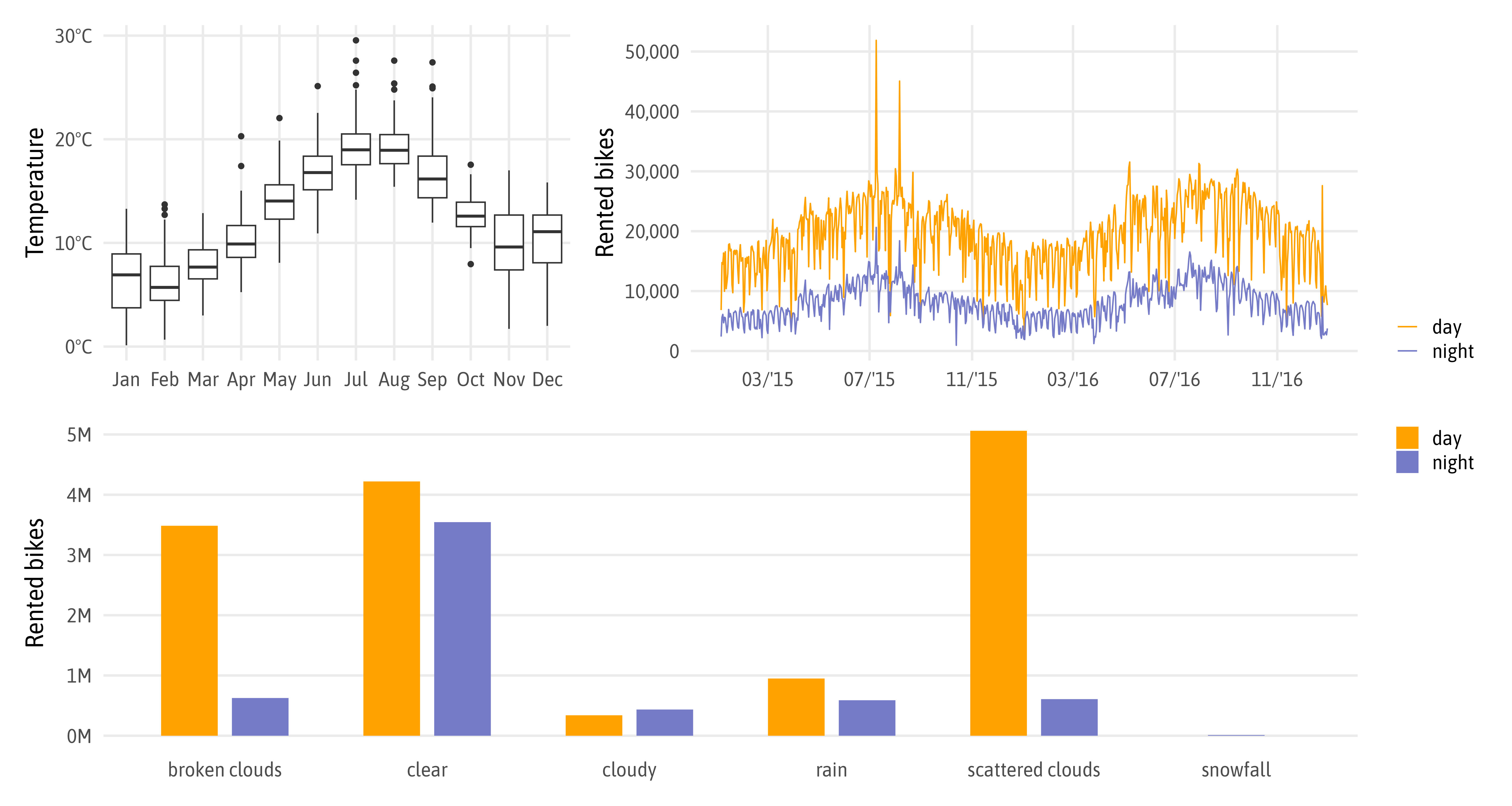
The final PNG graphic.