Engaging and Beautiful Data Visualizations with ggplot2

Working with Themes
— Exercise Solutions —

Cédric Scherer // posit::conf // September 2023

Exercise

Exercise

• Create a corporate or funny custom theme.
  • Make use of an existing complete theme to get started.
  • Pick a non-default font (or multiple) for your theme.
  • Optional: Try working with font variants.
  • Optional: Add other helpful arguments to your theme_* function.

Preparation

library(ggplot2)
library(readr)
library(dplyr)

Custom Theme

theme_bulls <- function(base_size = 18, base_family = "College Block", 
                        base_line_size = base_size/22, base_rect_size = base_size/22) {
  
  theme_bw(base_size = base_size, base_family = base_family, 
           base_line_size = base_line_size, base_rect_size = base_rect_size) + 
    theme( 
      plot.title = element_text(size = rel(2), color = "white", margin = margin(b = base_size/2)),
      plot.subtitle = element_text(margin = margin(t = -base_size/4, b = base_size/2)),
      plot.caption = element_text(color = "black", size = rel(.7), hjust = 0),
      plot.title.position = "plot",
      plot.caption.position = "plot",
      axis.title = element_text(color = "white"),
      axis.title.x = element_text(hjust = 1, margin = margin(t = base_size/2)),
      axis.title.y = element_text(hjust = 1, margin = margin(r = base_size/2)),
      axis.text = element_text(color = "black"),
      axis.ticks = element_line(color = "black"),
      panel.background = element_rect(fill = "#dfbb85", color = "white", linewidth = base_size/4), 
      panel.border = element_rect(fill = NA, color = "black", linewidth = base_size/10), 
      plot.background = element_rect(fill = "#CE1141", color = "black", linewidth = base_size/4), 
      legend.background = element_rect(fill = "transparent", color = "black"),
      legend.justification = "top",
      strip.text = element_text(size = rel(1.25), color = "white"),
      panel.grid.major = element_line(color = "white"),
      panel.grid.minor = element_blank(),
      plot.margin = margin(rep(base_size, 4))
    )
}

Apply Theme

data <- read_csv("https://query.data.world/s/cejs4o4gdt6autofsse7whhqnnmaii?dws=00000")

ggplot(filter(data, Team == "Chicago"), aes(x = Pts, y = Reb)) +
  geom_point(shape = "🏀", size = 5) +
  labs(title = "Let's Go Bulls! ⛹️️", x = "Points scored", y = "Rebounds", 
       caption = "Data: hoopsstats.com") +
  theme_bulls()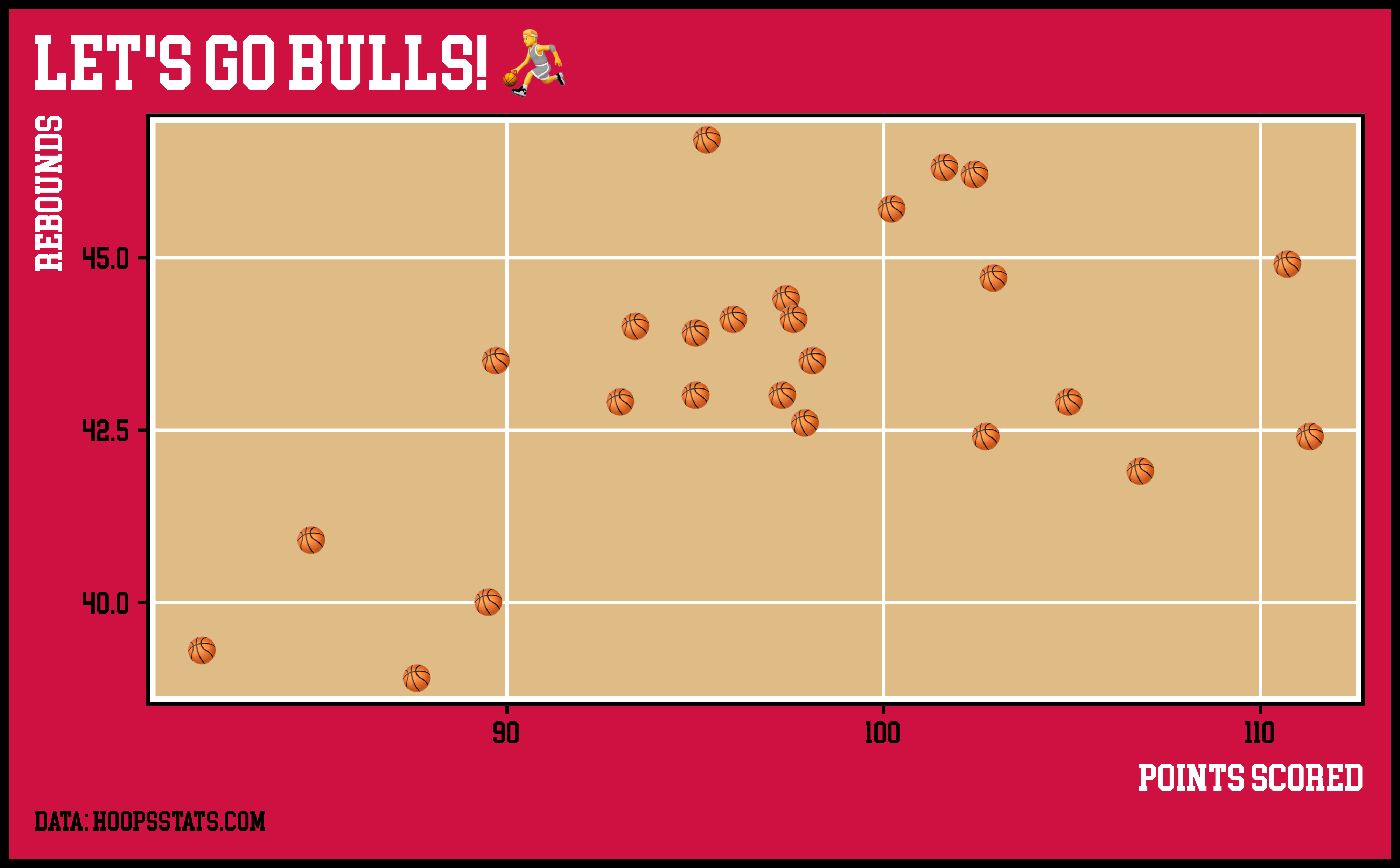

Custom Theme

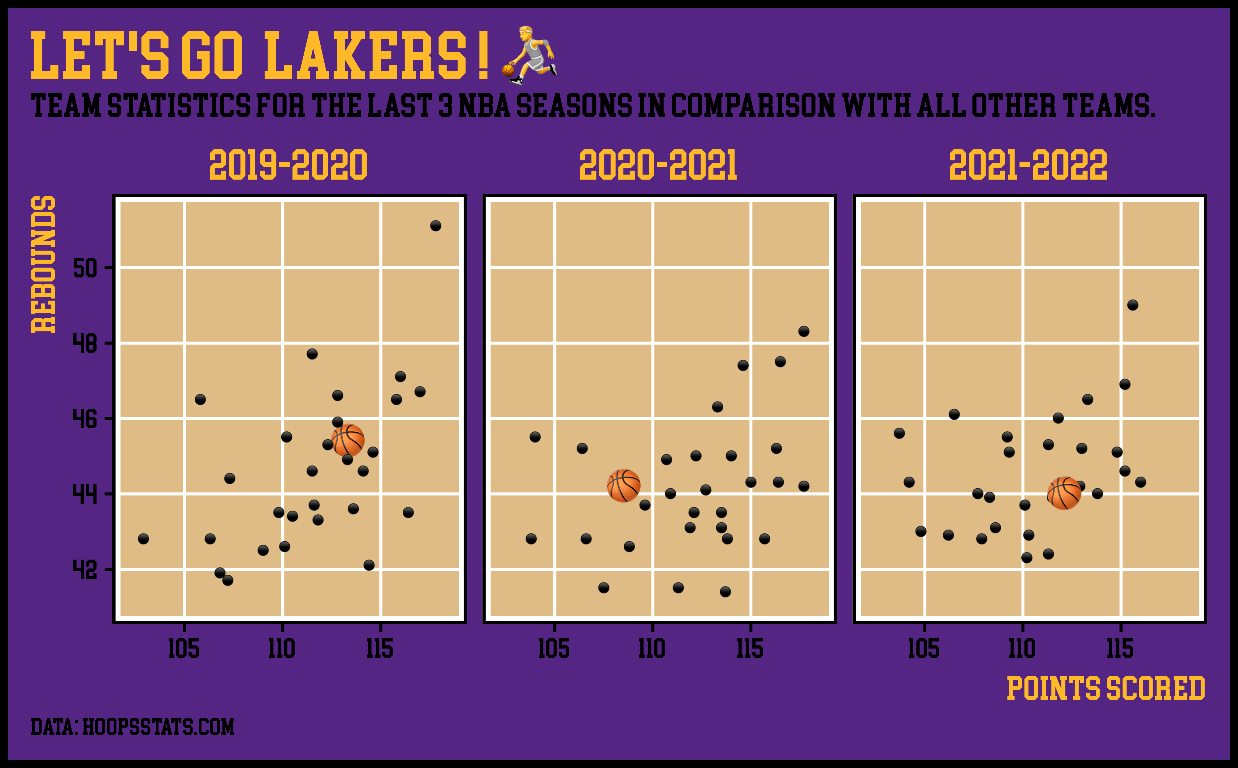
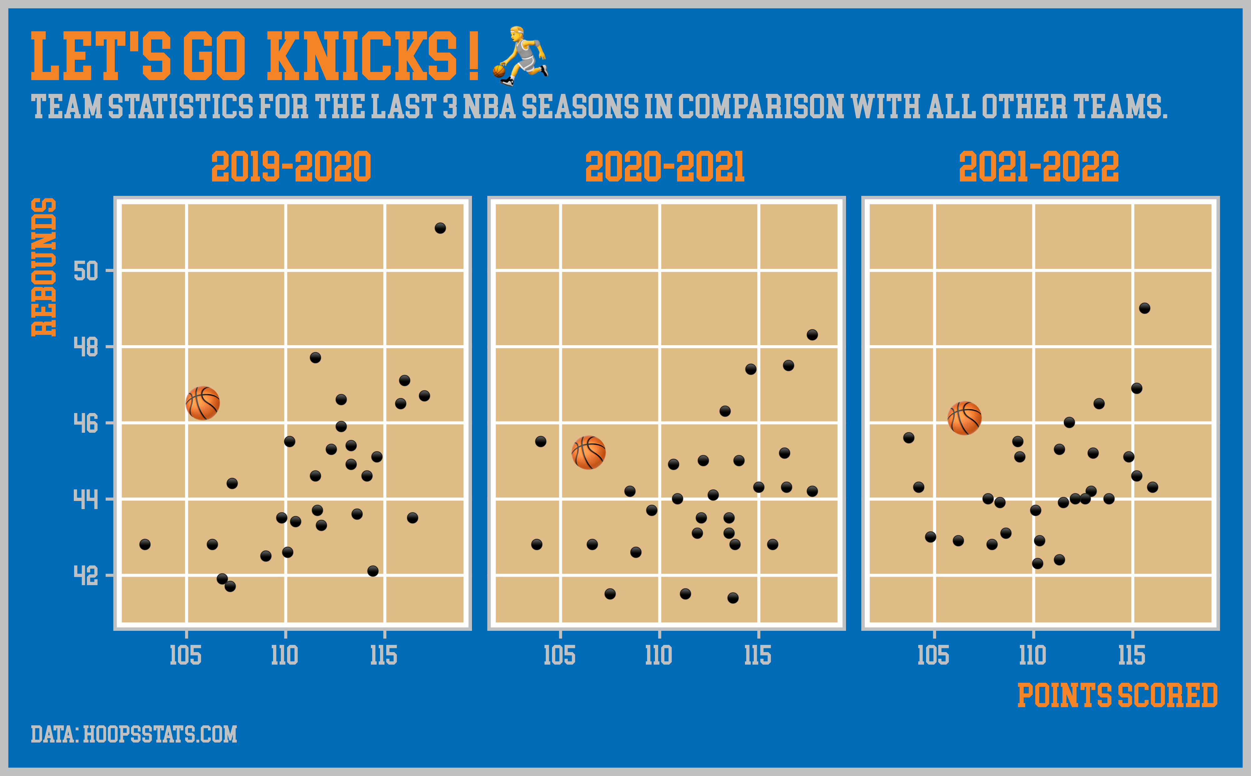
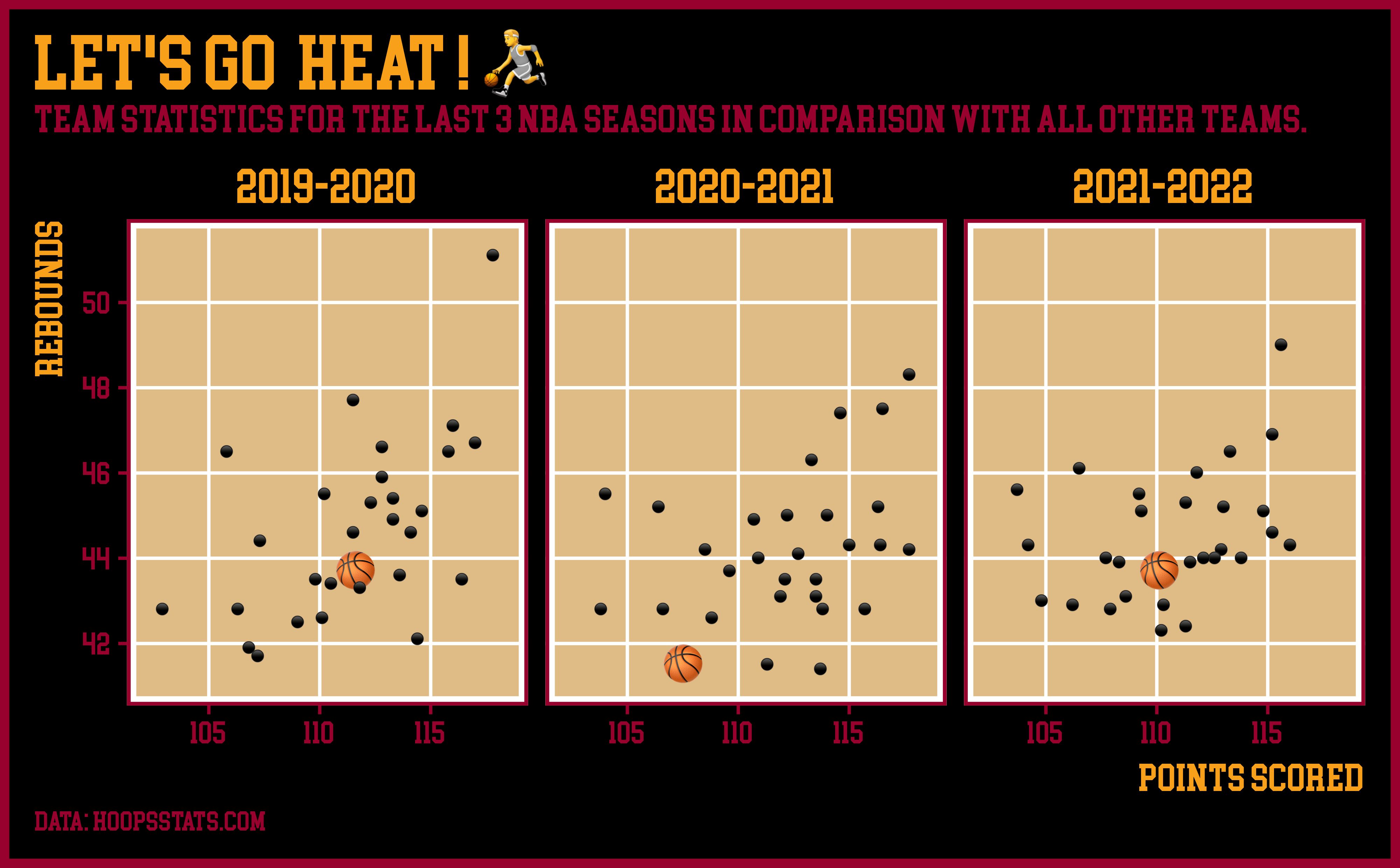
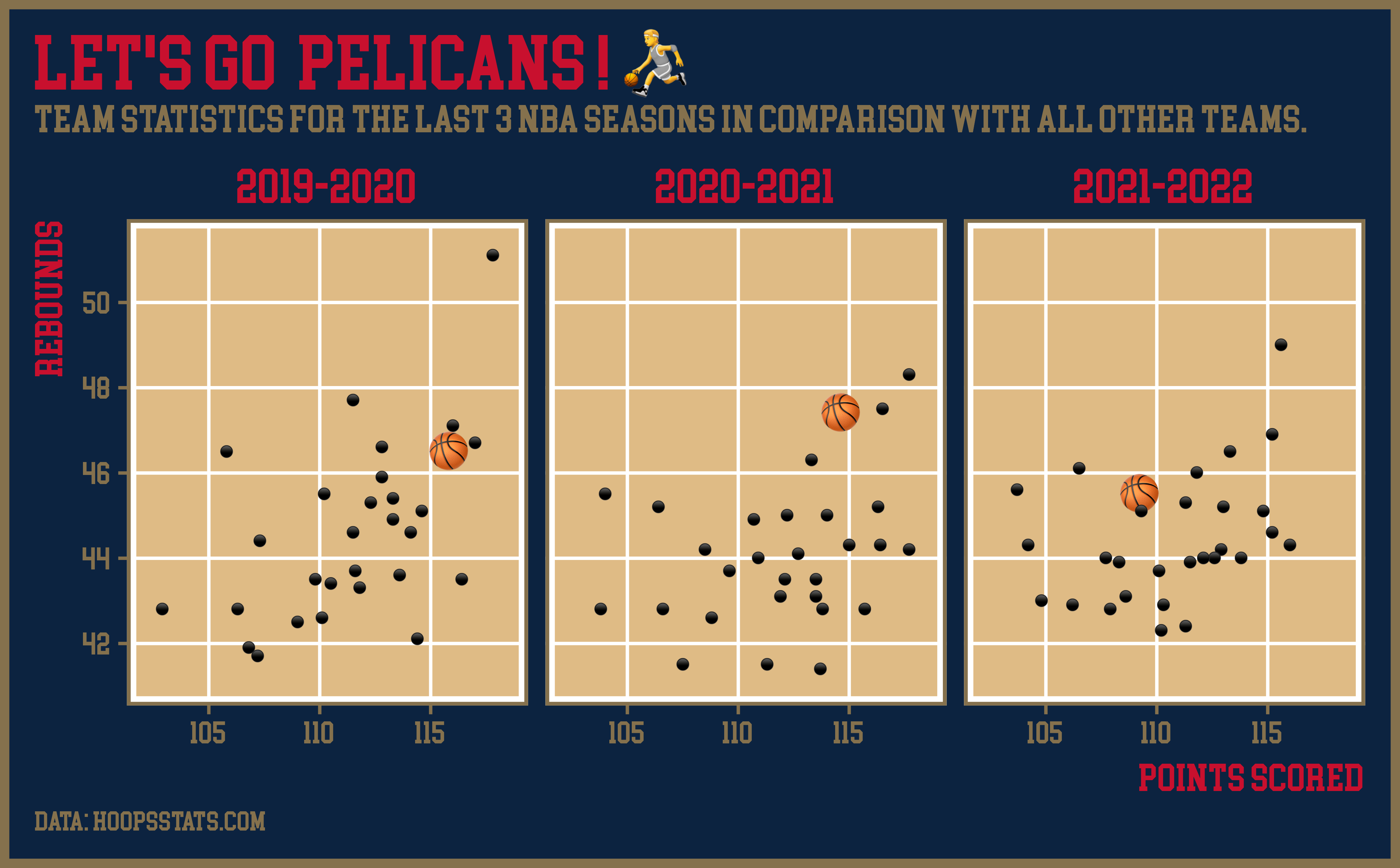
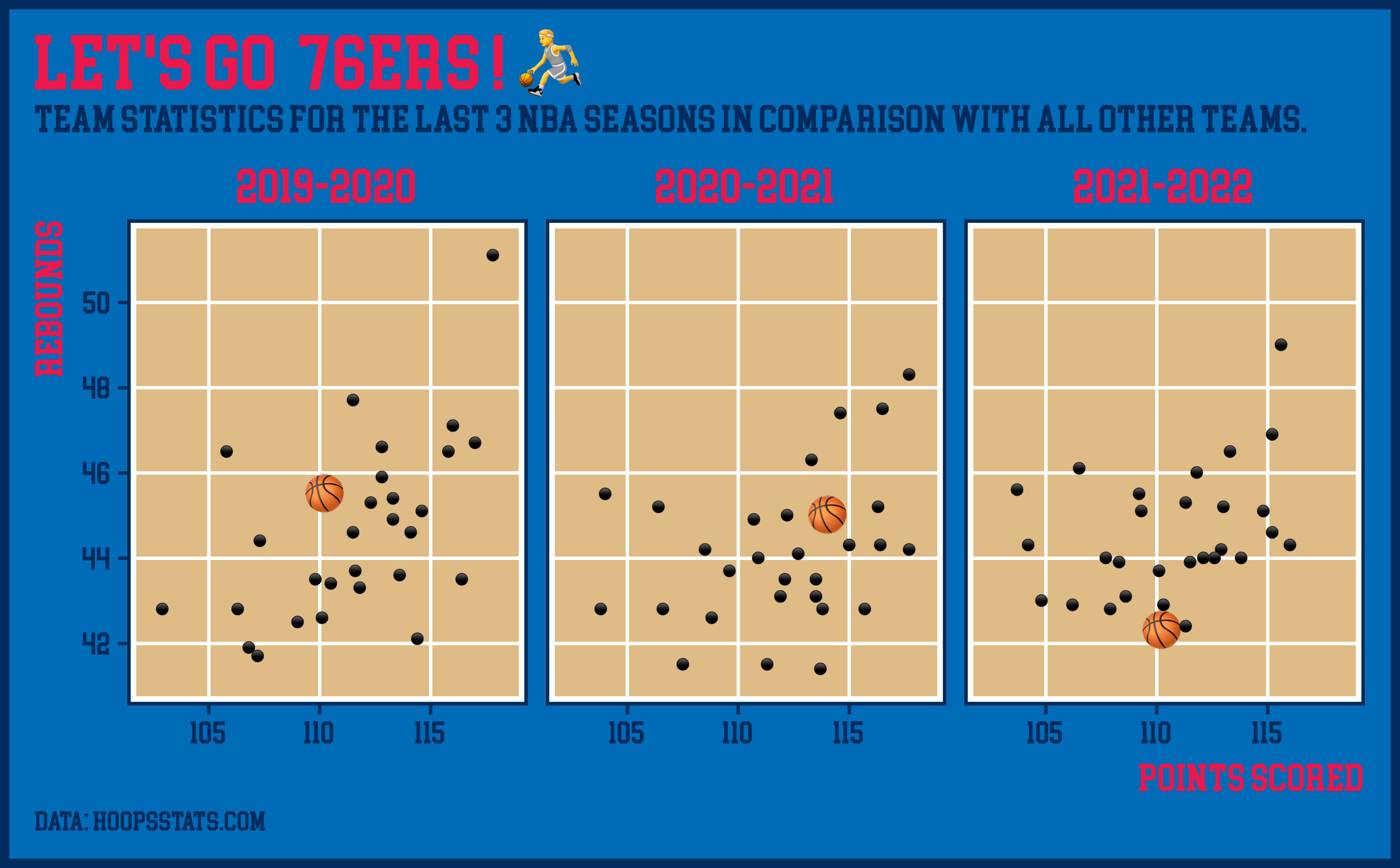
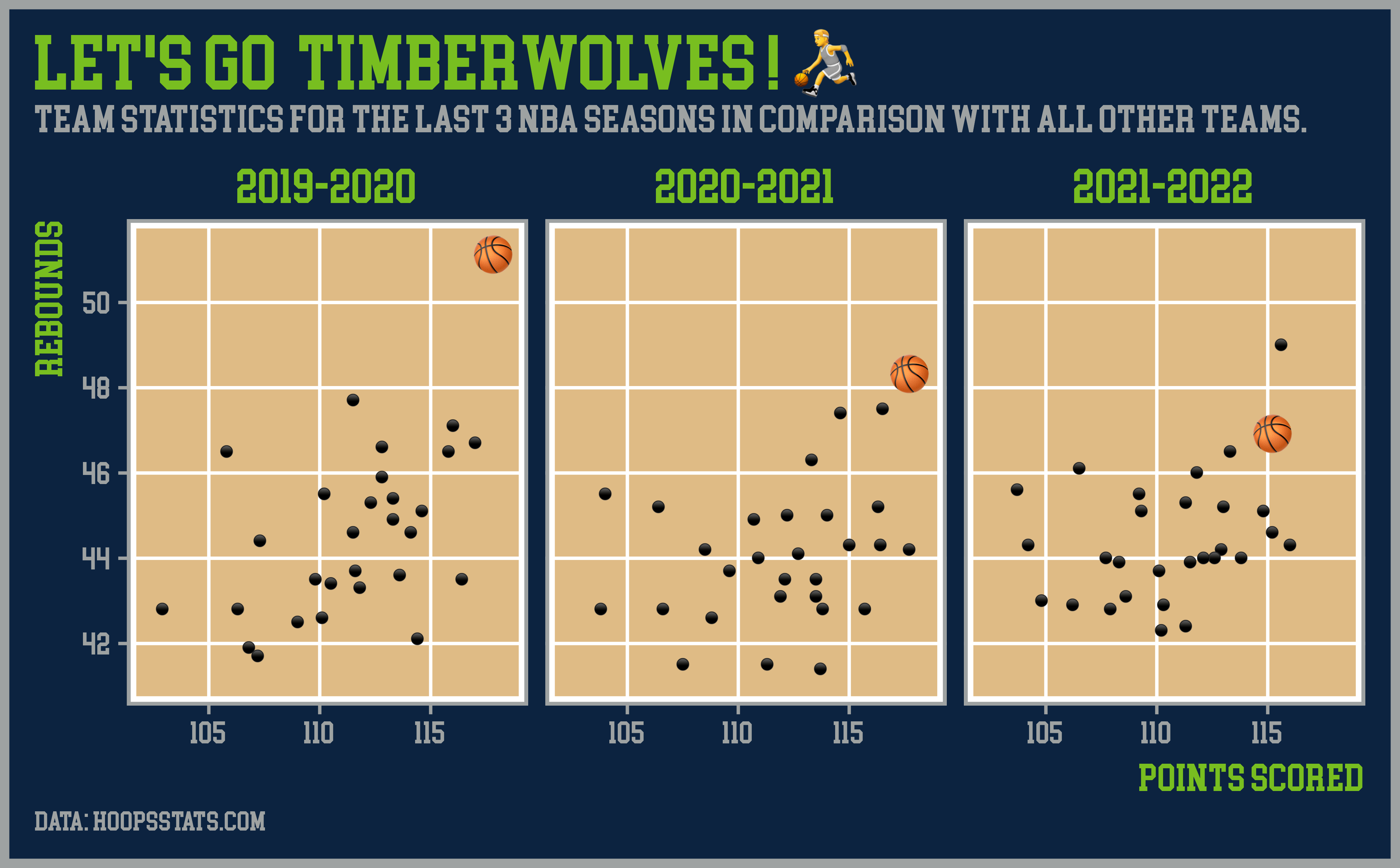
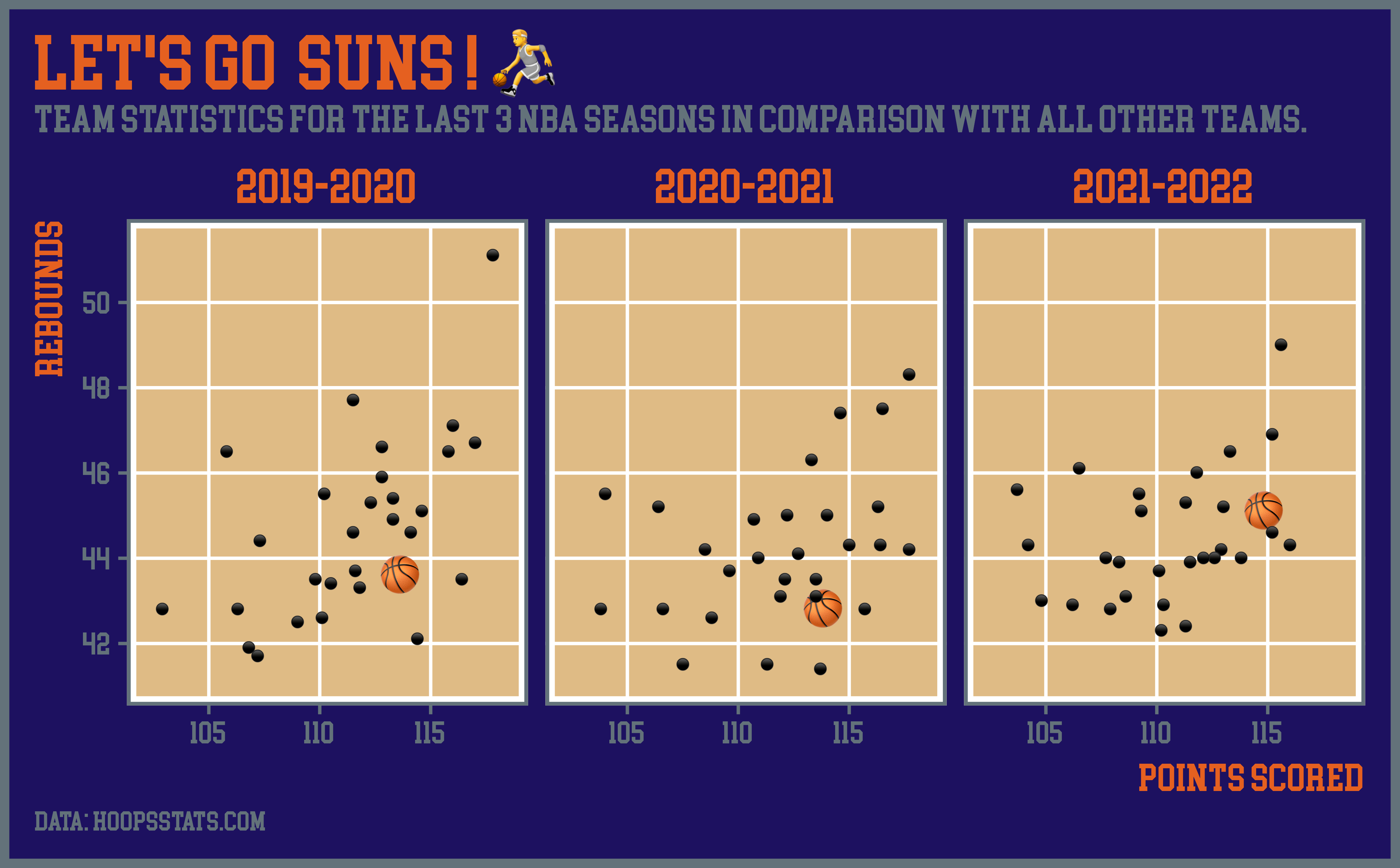
theme_nba <- function(base_size = 18, base_family = "College Block", 
                      base_line_size = base_size/22, base_rect_size = base_size/22,
                      team = "Bulls") {
  
  if(!team %in% c("Bulls", "Lakers", "Nuggets", "Celtics", "Knicks", "Heat", "Hornets", "Sixers", "Timberwolves", "Pelicans", "Suns")) stop('team should be one of "Bulls", "Lakers", "Nuggets", "Celtics", "Knicks", "Heat", "Hornets", "Sixers", "Timberwolves", "Pelicans", or "Suns".')
  
  colors <- data.frame(
    Bulls = c("#CE1141", "#FFFFFF", "#000000"),
    Lakers = c("#552583", "#FDB927", "#000000"),
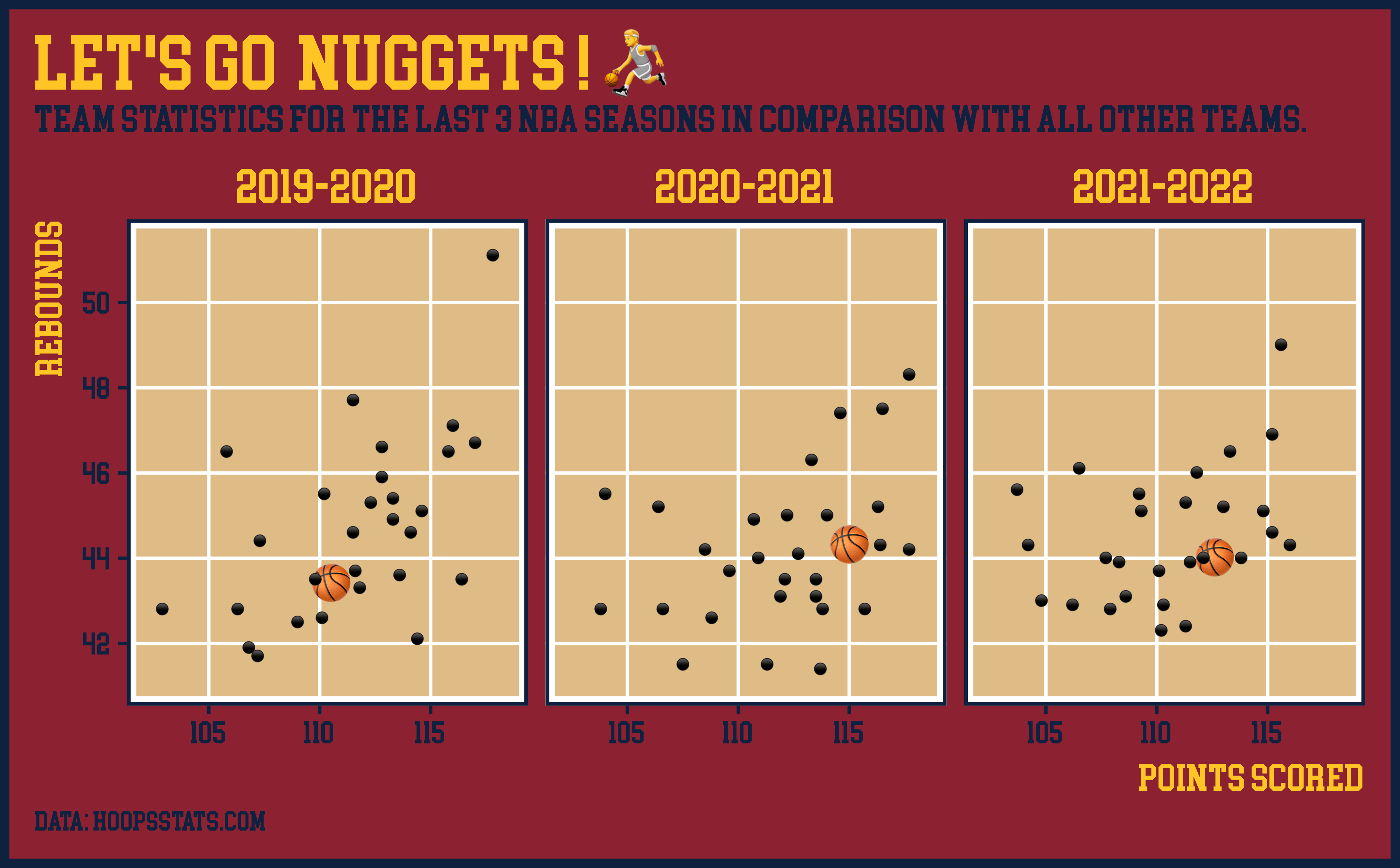
    Nuggets = c("#8B2131", "#FEC524", "#0E2240"),
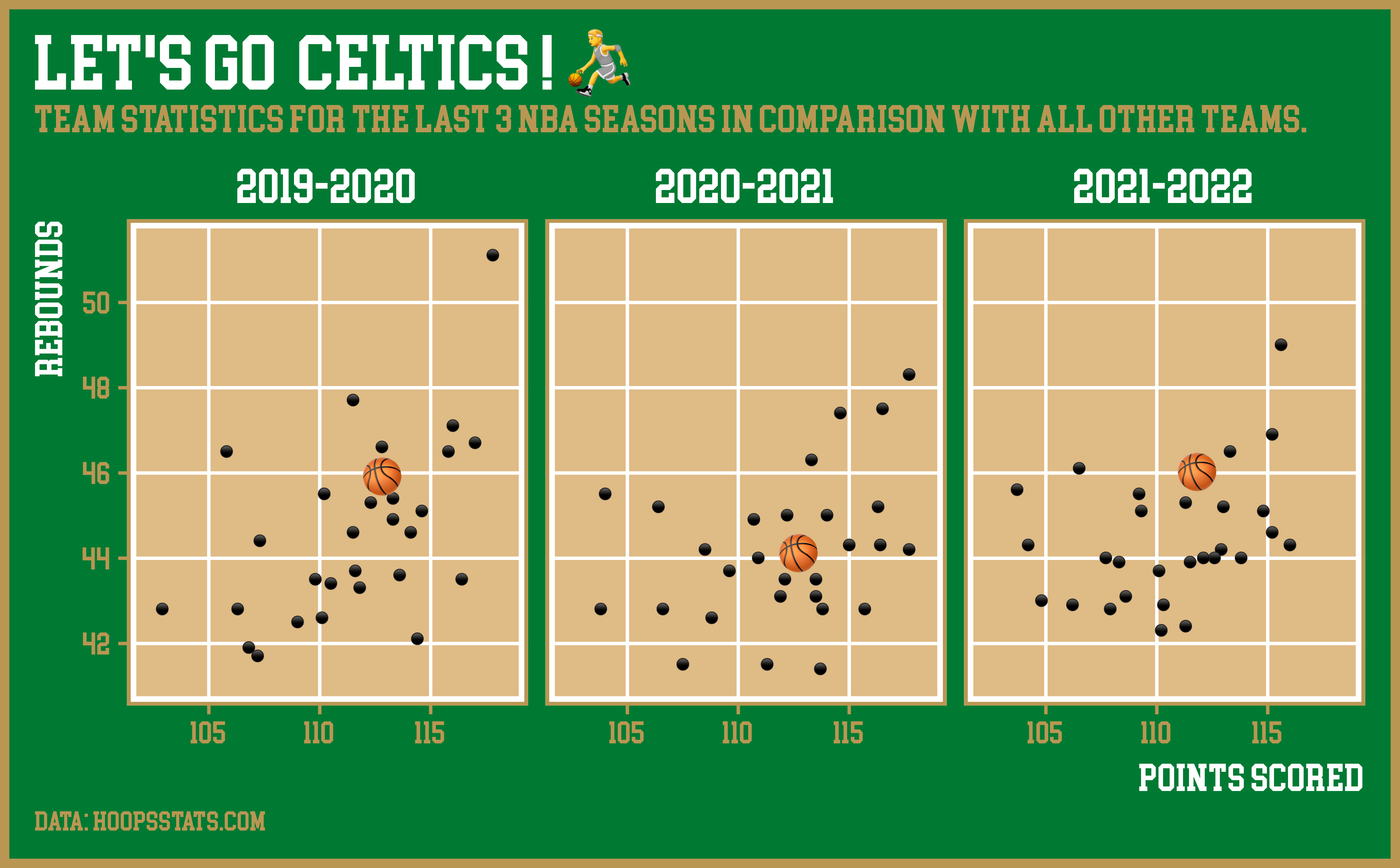
    Celtics = c("#007A33", "#FFFFFF", "#BA9653"),
    Knicks = c("#006BB6", "#F58426", "#BEC0C2"),
    Heat = c("#000000", "#F9A01B", "#98002E"),
    Hornets = c("#1D1160", "#A1A1A4", "#00788C"),
    Sixers = c("#006BB6", "#ED174C", "#002B5C"),
    Timberwolves = c("#0C2340", "#78BE20", "#9EA2A2"),
    Pelicans = c("#0C2340", "#C8102E", "#85714D"),
    Suns = c("#1D1160", "#E56020", "#63727A")
  )
  colors <- unname(colors[, team])
  
  theme_minimal(base_size = base_size, base_family = base_family, 
           base_line_size = base_line_size, base_rect_size = base_rect_size) + 
    theme( 
      plot.title = element_text(size = rel(2), color = colors[2], margin = margin(b = base_size/2)),
      plot.subtitle = element_text(color = colors[3], margin = margin(t = -base_size/4, b = base_size/2)),
      plot.caption = element_text(color = colors[3], size = rel(.7), hjust = 0),
      plot.title.position = "plot",
      plot.caption.position = "plot",
      axis.title = element_text(color = colors[2]),
      axis.title.x = element_text(hjust = 1, margin = margin(t = base_size/2)),
      axis.title.y = element_text(hjust = 1, margin = margin(r = base_size/2)),
      axis.text = element_text(color = colors[3]),
      axis.ticks = element_line(color = colors[3]),
      panel.background = element_rect(fill = "#dfbb85", color = "white", linewidth = base_size/4), 
      panel.border = element_rect(fill = NA, color = colors[3], linewidth = base_size/10), 
      plot.background = element_rect(fill = colors[1], color = colors[3], linewidth = base_size/4), 
      legend.background = element_rect(fill = "transparent", color = colors[3]),
      legend.justification = "top",
      strip.text = element_text(size = rel(1.25), color = colors[2]),
      panel.grid.major = element_line(color = "white"),
      panel.grid.minor = element_blank(),
      plot.margin = margin(rep(base_size, 4))
    )
}